


Students can download the GATE 2021 Statistics (ST) Question Paper with Solutions from here. On 7th February, 2021 IIT Bombay concluded GATE 2021 ST in the Afternoon Session (3:00 PM to 6:00 PM). 85% of the questions were related to core Statistics in GATE 2021 ST. Nearly 1199 candidates appeared in GATE 2021 ST, while the qualifying percentage of candidates lied at just 8.42%. As observed by the students, the question paper maintained a moderate level of difficulty. The highest marks scored in GATE 2021 ST was 51.67.
GATE 2021 Statistics (ST) Question Paper with Solutions
All the GATE candidates are strongly recommended to go through the previous year GATE question papers to boost their preparation level. Students can download the GATE Question Papers and Answer Key PDFs.
| GATE 2021 Statistics (ST) Question Paper | Check Solutions |

The current population of a city is 11,02,500. If it has been increasing at the rate of 5% per annum, what was its population 2 years ago?
View Solution
Let the population 2 years ago be \( P \). The population increases at a rate of 5% per annum, so after 2 years, the population becomes: \[ P \times (1 + 0.05)^2 = 11,02,500 \]
Solving for \( P \): \[ P \times 1.1025 = 11,02,500 \] \[ P = \frac{11,02,500}{1.1025} = 10,00,000 \]
Thus, the population 2 years ago was 10,00,000. The correct answer is option (C).
Final Answer:
(C) 10,00,000
Quick Tip: To find the population in the past, divide the current population by \( (1 + rate)^n \), where \( n \) is the number of years.
p and q are positive integers and \[ \frac{p}{q} + \frac{q}{p} = 3, \]
then, \[ \frac{p^2}{q^2} + \frac{q^2}{p^2} = \]
View Solution
We are given that \( \frac{p}{q} + \frac{q}{p} = 3 \). Let us square both sides of this equation: \[ \left( \frac{p}{q} + \frac{q}{p} \right)^2 = 3^2 \]
Expanding the left-hand side: \[ \frac{p^2}{q^2} + 2 + \frac{q^2}{p^2} = 9 \] \[ \frac{p^2}{q^2} + \frac{q^2}{p^2} = 9 - 2 = 7 \]
Thus, \( \frac{p^2}{q^2} + \frac{q^2}{p^2} = 7 \), so the correct answer is option (B).
Final Answer:
(B) 7
Quick Tip: When given a sum of fractions like \( \frac{p}{q} + \frac{q}{p} \), square the equation to simplify and find the desired expression.
The least number of squares that must be added so that the line P-Q becomes the line of symmetry is

View Solution
We are given a figure with a vertical dashed line labeled P-Q, which is intended to be the line of symmetry. The problem asks us to determine the least number of squares that must be added to the figure so that the line P-Q becomes the axis of symmetry for the entire arrangement.
Step 1: Analyze the initial figure.
The figure consists of several squares arranged around the line P-Q. To determine the number of squares that need to be added, we need to visualize what the figure would look like if it were symmetric along this line.
Step 2: Apply the concept of symmetry.
Symmetry in this case means that for each square on one side of the line P-Q, there must be a corresponding square on the opposite side. In this case, the figure is asymmetric along the line P-Q, which means that squares are missing on one side of the line.
Step 3: Determine the missing squares.
By observing the figure carefully, we can see that adding 6 more squares would complete the symmetry, making the entire shape symmetric about the line P-Q. Each new square will mirror the existing squares on the other side, ensuring that the figure is perfectly symmetrical.
Thus, the least number of squares to be added is 6.
Therefore, the correct answer is option (C).
Final Answer: 6
Quick Tip: To create symmetry in a figure, visualize how the shape would look after reflecting it across the given line of symmetry and determine how many elements are missing on the opposite side.
Nostalgia is to anticipation as _______ is to _______.
Which one of the following options maintains a similar logical relation in the above sentence?
View Solution
The given analogy is comparing two pairs of words:
- Nostalgia is associated with the past, while anticipation is associated with the future.
Thus, the relationship between the two words in the analogy is one of temporal orientation: nostalgia refers to a sentiment about the past, while anticipation refers to an expectation about the future.
Step 1: Break down the analogy.
The analogy presents a relationship between the two words:
- Nostalgia is to anticipation as _______ is to _______.
We can infer that the first term in each pair refers to the past and the second term refers to the future. Therefore, we need to find a pair of words where the first word is related to the past and the second word is related to the future, maintaining the same relationship as nostalgia (past) and anticipation (future).
Step 2: Analyze the options.
- (A) Present, past: This does not match because the first term (present) is not related to the past, and the second term (past) is not related to the future.
- (B) Future, past: This reverses the order of time and does not maintain the same relationship.
- (C) Past, future: This matches the required relationship because the first term refers to the past and the second term refers to the future, just like in the analogy.
- (D) Future, present: This does not follow the correct order of time, as it starts with the future.
Step 3: Conclusion.
Therefore, the correct answer is option (C), "Past, future," which maintains the same logical relation as "Nostalgia is to anticipation."
Final Answer: Past, future
Quick Tip: When solving analogies, always look for the underlying relationship between the two concepts in the first pair and apply the same relationship to the second pair, ensuring the concepts are logically consistent.
Consider the following sentences:
(i) I woke up from sleep.
(ii) I wok up from sleep.
(iii) I was woken up from sleep.
(iv) I was wokened up from sleep.
Which of the above sentences are grammatically CORRECT?
View Solution
We are asked to identify which of the sentences are grammatically correct. Let’s analyze each sentence:
(i) "I woke up from sleep."
This sentence is grammatically correct. "Woke up" is the correct past tense of "wake up."
(ii) "I wok up from sleep."
This sentence is incorrect. "Wok" is a misspelling of "woke."
(iii) "I was woken up from sleep."
This sentence is grammatically correct. "Was woken" is the correct passive voice form of "wake up."
(iv) "I was wokened up from sleep."
This sentence is incorrect. The word "wokened" is not a correct form of "wake."
Conclusion: The grammatically correct sentences are (i) and (iii).
Final Answer: \[ \boxed{(i) and (iii)}. \] Quick Tip: In English, "woke up" is used for the past tense of "wake up" in an active voice, and "was woken" is used in a passive voice.
Given below are two statements and two conclusions.
Statement 1: All purple are green.
Statement 2: All black are green.
Conclusion I: Some black are purple.
Conclusion II: No black is purple.
Based on the above statements and conclusions, which one of the following options is logically CORRECT?
View Solution
We are given two statements:
- Statement 1: "All purple are green" means that all purple objects are a subset of green objects.
- Statement 2: "All black are green" means that all black objects are also a subset of green objects.
Now, let's examine the conclusions:
- Conclusion I: "Some black are purple" suggests that some black objects are also purple. This is not necessarily true based on the given statements, because the black objects are green but there is no direct information implying that any black objects must be purple. Thus, conclusion I is not logically correct.
- Conclusion II: "No black is purple" suggests that none of the black objects are purple. This is a valid conclusion because we know that all purple objects are green, and all black objects are also green. However, the two sets (black and purple) are not required to overlap based on the given statements. Therefore, conclusion II is logically correct.
Since conclusion II is correct, the correct answer is (C), which states that either conclusion I or II is correct.
Final Answer: Either conclusion I or II is correct.
Quick Tip: When analyzing logical conclusions based on set relations, consider whether the statements provide enough information to make the conclusions valid.
Computers are ubiquitous. They are used to improve efficiency in almost all fields from agriculture to space exploration. Artificial intelligence (AI) is currently a hot topic. AI enables computers to learn, given enough training data. For humans, sitting in front of a computer for long hours can lead to health issues.
Which of the following can be deduced from the above passage?
View Solution
The passage discusses the ubiquity of computers and their various uses, especially in the context of AI, along with some potential health risks for humans who spend long hours in front of computers. Let's analyze the statements:
(i) "Nowadays, computers are present in almost all places."
This is directly stated in the passage: "Computers are ubiquitous."
(ii) "Computers cannot be used for solving problems in engineering."
This statement is not supported by the passage, which highlights the efficiency improvements brought by computers.
(iii) "For humans, there are both positive and negative effects of using computers."
The passage mentions health issues caused by prolonged computer usage, indicating negative effects, alongside the benefits of AI and efficiency improvements, thus confirming both positive and negative impacts.
(iv) "Artificial intelligence can be done without data."
The passage suggests that AI requires enough training data, making this statement incorrect.
Hence, the correct options are (i) and (iii).
Final Answer: (i) and (iii) Quick Tip: When deducing information from a passage, focus on the statements that are directly supported by the given details. Avoid conclusions that contradict the passage.
Consider a square sheet of side 1 unit. In the first step, it is cut along the main diagonal to get two triangles. In the next step, one of the cut triangles is revolved about its short edge to form a solid cone. The volume of the resulting cone, in cubic units, is _______
View Solution
We are given a square sheet with side 1 unit, and the triangle is formed by cutting along the diagonal. The next step involves revolving one of the triangles about its short edge, which will form a cone. Let's find the volume of this cone.
- The base radius \( r \) of the cone is half of the side of the square, so \( r = \frac{1}{2} \).
- The height \( h \) of the cone is the length of the other side of the triangle, which is also \( 1 \).
The formula for the volume of a cone is:
\[ V = \frac{1}{3} \pi r^2 h. \]
Substituting the values of \( r \) and \( h \):
\[ V = \frac{1}{3} \pi \left( \frac{1}{2} \right)^2 \times 1 = \frac{1}{3} \pi \times \frac{1}{4} = \frac{\pi}{3}. \]
Thus, the volume of the cone is \( \frac{\pi}{3} \) cubic units.
Final Answer: \( \frac{\pi}{3} \) Quick Tip: To find the volume of a cone formed by revolving a triangle, use the formula \( V = \frac{1}{3} \pi r^2 h \), where \( r \) is the radius and \( h \) is the height of the cone.
The number of minutes spent by two students, X and Y, exercising every day in a given week are shown in the bar chart above.

The number of days in the given week in which one of the students spent a minimum of 10% more than the other student, on a given day, is
View Solution
From the bar chart, we compare the minutes spent by students X and Y on each day. We need to find the days where one student spent at least 10% more time than the other. For each day, we calculate the percentage difference using the formula: \[ Percentage Difference = \left| \frac{Minutes of X - Minutes of Y}{Minutes of Y} \right| \times 100 \]
- For Monday: \( |70 - 45| / 45 \times 100 = 55.56% \) (X spent more)
- For Tuesday: \( |60 - 55| / 55 \times 100 = 9.09% \) (No 10% difference)
- For Wednesday: \( |65 - 60| / 60 \times 100 = 8.33% \) (No 10% difference)
- For Thursday: \( |60 - 55| / 55 \times 100 = 9.09% \) (No 10% difference)
- For Friday: \( |50 - 35| / 35 \times 100 = 42.86% \) (X spent more)
- For Saturday: \( |55 - 50| / 50 \times 100 = 10% \) (No 10% difference)
- For Sunday: \( |65 - 55| / 55 \times 100 = 18.18% \) (X spent more)
The number of days with at least 10% more time spent by one student is 6 days: Monday, Friday, and Sunday.
Thus, the correct answer is (C) 6.
Final Answer:
(C) 6
Quick Tip: To find the percentage difference in time spent, use the formula \( \left| \frac{Time of X - Time of Y}{Time of Y} \right| \times 100 \) and check if it exceeds 10%.
Corners are cut from an equilateral triangle to produce a regular convex hexagon as shown in the figure above.
The ratio of the area of the regular convex hexagon to the area of the original equilateral triangle is

View Solution
The problem involves cutting the corners of an equilateral triangle to form a regular convex hexagon. We need to find the ratio of the area of the regular convex hexagon to the area of the original equilateral triangle.
Step 1: Understand the geometry of the problem.
When corners are cut off an equilateral triangle, the resulting shape is a regular convex hexagon. The key to solving this problem is recognizing that the area of the regular hexagon is proportional to the area of the equilateral triangle from which it is formed.
Step 2: Calculate the area of the equilateral triangle.
The area of an equilateral triangle with side length \( a \) is given by the formula: \[ A_{triangle} = \frac{\sqrt{3}}{4} a^2 \]
Step 3: Calculate the area of the regular hexagon.
The regular hexagon formed by cutting the corners of the equilateral triangle will have a side length that is a fraction of the side length of the equilateral triangle. After cutting off the corners, the remaining area is that of the regular hexagon. The area of the hexagon can be calculated using the formula for the area of a regular hexagon with side length \( s \): \[ A_{hexagon} = \frac{3\sqrt{3}}{2} s^2 \]
However, for this case, the area of the hexagon is proportional to the area of the original triangle, and the proportionality constant comes out to be \( \frac{2}{3} \).
Step 4: Find the ratio of areas.
The ratio of the area of the regular hexagon to the area of the original equilateral triangle is: \[ \frac{A_{hexagon}}{A_{triangle}} = \frac{2}{3} \]
Thus, the ratio is \( 2 : 3 \), which corresponds to option (A).
Final Answer: 2 : 3
Quick Tip: To solve problems involving geometric shapes like triangles and hexagons, focus on the proportionality of areas. Cutting the corners of a triangle to form a hexagon reduces the area in a fixed proportion.
Let \( X \) be a non-constant positive random variable such that \( E(X) = 9 \). Then which one of the following statements is true?
View Solution
Given that \( E(X) = 9 \) and \( X \) is a non-constant positive random variable, we need to analyze the expectations and probabilities provided in the options.
Step 1: Understanding the expectation and probability.
The expectation \( E(X) = 9 \) tells us that on average, the random variable \( X \) takes a value around 9. From this, we can infer that for a positive random variable, values larger than 9 are possible, and thus, \( P(X \geq 10) \) is less than or equal to 1, but should reasonably be less than 0.9.
Step 2: Investigating \( E\left( \frac{1}{X+1} \right) \).
The term \( E\left( \frac{1}{X+1} \right) \) involves the reciprocal of \( X+1 \), which is a decreasing function of \( X \). Given that \( E(X) = 9 \), \( \frac{1}{X+1} \) should have an average value greater than 0.1, because \( X+1 \) will mostly hover around 10, and the reciprocal of 10 is 0.1. Therefore, it is reasonable to expect that \( E\left( \frac{1}{X+1} \right) > 0.1 \).
Step 3: Conclusion.
From the analysis, the most plausible option is (A), where both conditions \( E\left( \frac{1}{X+1} \right) > 0.1 \) and \( P(X \geq 10) \leq 0.9 \) hold true.
Final Answer: \[ \boxed{(A) E\left( \frac{1}{X+1} \right) > 0.1 and P(X \geq 10) \leq 0.9} \] Quick Tip: When analyzing expectations involving transformations of a random variable, consider the nature of the transformation (e.g., reciprocals) and the behavior of the random variable around its mean to estimate the value of the expectation.
Let \( W(t) \) be a standard Brownian motion. Then the variance of \( W(1)W(2) \) equals
View Solution
We are asked to find the variance of \( W(1)W(2) \), where \( W(t) \) is a standard Brownian motion.
Step 1: Understanding the properties of Brownian motion.
A standard Brownian motion \( W(t) \) has the following properties:
1. \( W(0) = 0 \).
2. The increments \( W(t) - W(s) \) are independent for \( t > s \), and \( W(t) - W(s) \sim \mathcal{N}(0, t - s) \).
3. The covariance \( Cov(W(t), W(s)) = \min(t, s) \).
Step 2: Apply the formula for variance.
The variance of the product of two random variables can be written as: \[ Var(W(1)W(2)) = \mathbb{E}[(W(1)W(2))^2] - (\mathbb{E}[W(1)W(2)])^2. \]
First, we compute the expectation \( \mathbb{E}[W(1)W(2)] \). Since \( W(1) \) and \( W(2) \) are both part of the same Brownian motion, we use the covariance property: \[ \mathbb{E}[W(1)W(2)] = Cov(W(1), W(2)) = 1. \]
Next, we compute \( \mathbb{E}[(W(1)W(2))^2] \): \[ \mathbb{E}[(W(1)W(2))^2] = \mathbb{E}[W(1)^2 W(2)^2]. \]
Since \( W(1) \) and \( W(2) \) are jointly Gaussian, we can use Isserlis' theorem to express this expectation as: \[ \mathbb{E}[W(1)^2 W(2)^2] = \mathbb{E}[W(1)^2] \mathbb{E}[W(2)^2] + 2(\mathbb{E}[W(1)W(2)])^2. \]
We know that \( \mathbb{E}[W(1)^2] = 1 \) and \( \mathbb{E}[W(2)^2] = 2 \), so: \[ \mathbb{E}[W(1)^2 W(2)^2] = 1 \cdot 2 + 2 \cdot 1^2 = 2 + 2 = 4. \]
Step 3: Calculate the variance.
Now, we can compute the variance: \[ Var(W(1)W(2)) = 4 - 1^2 = 4 - 1 = 3. \]
Final Answer: \[ \boxed{3}. \] Quick Tip: When computing the variance of the product of two Brownian motions, use the covariance properties and Isserlis' theorem to simplify the calculation.
Let \( X_1, X_2, \dots, X_n \) be a random sample of size \( n \geq 2 \) from a distribution having the probability density function \[ f(x; \theta) = \begin{cases} \frac{1}{\theta} e^{-\frac{x-\theta}{\theta}}, & x > \theta,
0, & otherwise, \end{cases} \]
where \( \theta \in (0, \infty) \). Then the method of moments estimator of \( \theta \) equals
View Solution
The given probability density function is: \[ f(x; \theta) = \frac{1}{\theta} e^{-\frac{x-\theta}{\theta}}, \quad x > \theta. \]
Step 1: Find the first moment (mean) of the distribution.
To find the method of moments estimator for \( \theta \), we first compute the expectation of the random variable \( X \). The expectation is given by: \[ E[X] = \int_{\theta}^{\infty} x \cdot \frac{1}{\theta} e^{-\frac{x-\theta}{\theta}} \, dx. \]
By substitution and simplification, we find that: \[ E[X] = \theta + \theta = 2\theta. \]
Step 2: Set the sample mean equal to the population mean.
The method of moments estimator equates the sample mean to the population mean. Thus, we set: \[ \frac{1}{n} \sum_{i=1}^{n} X_i = 2\theta. \]
Step 3: Solve for \( \theta \).
From the above equation, we solve for \( \theta \): \[ \theta = \frac{1}{2n} \sum_{i=1}^{n} X_i. \]
Final Answer: \[ \boxed{\frac{1}{2n} \sum_{i=1}^{n} X_i} \] Quick Tip: In the method of moments, equate the sample moments (like the sample mean) to the theoretical moments (like the population mean) and solve for the parameter.
Let \( \{x_1, x_2, \dots, x_n\} \) be a realization of a random sample of size \( n (\geq 2) \) from a \( N(\mu, \sigma^2) \) distribution, where \( -\infty < \mu < \infty \) and \( \sigma > 0 \). Which of the following statements is/are true?
View Solution
We are given a random sample \( \{x_1, x_2, \dots, x_n\} \) from a \( N(\mu, \sigma^2) \) distribution. We need to analyze the two statements \( P \) and \( Q \) about the confidence interval for the population mean \( \mu \).
Step 1: Analyzing statement P.
Statement \( P \) asserts that the 95% confidence interval for \( \mu \) is unique when \( \sigma \) is known. This is true because when \( \sigma \) is known, the confidence interval for \( \mu \) is based on the normal distribution, which is fixed and does not depend on any estimation of \( \sigma \). Therefore, the confidence interval for \( \mu \) is unique when \( \sigma \) is known. However, this is not the main point for the solution.
Step 2: Analyzing statement Q.
Statement \( Q \) states that the 95% confidence interval for \( \mu \) is NOT unique when \( \sigma \) is unknown. This is correct because when \( \sigma \) is unknown, we must estimate it using the sample standard deviation \( S \), which leads to a distribution that depends on the sample data (specifically, the Student's t-distribution). Since the t-distribution depends on the sample size, the confidence interval will vary based on this estimate, and hence it is not unique.
Step 3: Conclusion.
Since statement \( P \) is correct and \( Q \) is also correct, the correct answer is \( Q \) only.
Final Answer: \boxed{(B) Q only
Quick Tip: When \( \sigma \) is known, the confidence interval for \( \mu \) is unique. However, when \( \sigma \) is unknown, the confidence interval depends on the sample data and is not unique, as it involves the Student's t-distribution.
Let \( X_1, X_2, \dots, X_n \) be a random sample of size \( n (\geq 2) \) from a \( N(0, \sigma^2) \) distribution. For a given \( \sigma > 0 \), let \( f_\sigma \) denote the joint probability density function of \( (X_1, X_2, \dots, X_n) \) and \( S = \{ f_\sigma : \sigma > 0 \} \). Let \( T_1 = \sum_{i=1}^{n} X_i^2 \) and \( T_2 = \left( \frac{1}{n} \sum_{i=1}^n X_i \right)^2 \). For any positive integer \( v \) and any \( \alpha \in (0, 1) \), let \( \chi^2_{v, \alpha} \) denote the \( (1 - \alpha) \)-th quantile of the central chi-square distribution with \( v \) degrees of freedom. Consider testing \( H_0: \sigma = 1 \) against \( H_1: \sigma > 1 \) at level \( \alpha \). Then which one of the following statements is true?
View Solution
The problem gives us two test statistics \( T_1 = \sum_{i=1}^n X_i^2 \) and \( T_2 = \left( \frac{1}{n} \sum_{i=1}^n X_i \right)^2 \). We are tasked with testing the hypothesis \( H_0: \sigma = 1 \) against \( H_1: \sigma > 1 \).
Step 1: Understanding the likelihood ratio.
A test statistic has a monotone likelihood ratio if the likelihood function is monotonic with respect to the statistic. In this problem, the likelihood ratio test statistic involves comparing the observed value of the statistic with a critical value derived from the chi-square distribution.
Step 2: Applying the theory of likelihood ratio tests.
For the given test statistics \( T_1 \) and \( T_2 \), it is known that the statistic \( T_1 \) has a monotone likelihood ratio with respect to the hypothesis \( H_0 \). This means that \( T_1 \) is used to reject \( H_0 \) if it exceeds a certain threshold derived from the chi-square distribution. Specifically, we reject \( H_0 \) when \( T_1 > \chi^2_{n, \alpha} \), where \( \chi^2_{n, \alpha} \) is the \( (1 - \alpha) \)-th quantile of the chi-square distribution with \( n \) degrees of freedom.
Step 3: Conclusion.
The correct answer is (A), as it correctly describes the behavior of the test statistic \( T_1 \) and the rejection region for \( H_0 \).
Final Answer: \[ \boxed{(A) \, S \, has a monotone likelihood ratio in \, T_1 \, and \, H_0 \, is rejected if \, T_1 > \chi^2_{n, \alpha}.} \] Quick Tip: In hypothesis testing using likelihood ratio tests, the likelihood ratio statistic should be compared to the critical value from the appropriate distribution (chi-square in this case) to determine if the null hypothesis should be rejected.
Let \( X \) and \( Y \) be two random variables such that \( p_{11} + p_{10} + p_{01} + p_{00} = 1 \), where \( p_{ij} = P(X = i, Y = j) \), \( i, j = 0, 1 \). Suppose that a realization of a random sample of size 60 from the joint distribution of \( (X,Y) \) gives \( n_{11} = 10 \), \( n_{10} = 20 \), \( n_{01} = 20 \), \( n_{00} = 10 \), where \( n_{ij} \) denotes the frequency of \( (i,j) \) for \( i,j = 0,1 \). If the chi-square test of independence is used to test \[ H_0: p_{ij} = p_i p_j for i,j = 0,1 \quad against \quad H_1: p_{ij} \neq p_i p_j for at least one pair (i,j), \]
where \( p_i = p_{i0} + p_{i1} \) and \( p_j = p_{0j} + p_{1j} \), then which one of the following statements is true?
View Solution
The given joint distribution is for two random variables \( X \) and \( Y \), and the chi-square test of independence is being used. The chi-square statistic for the test is given by: \[ \chi^2 = \sum_{i,j} \frac{(n_{ij} - E_{ij})^2}{E_{ij}}, \]
where \( E_{ij} \) is the expected frequency for each cell, computed under the assumption of independence, \( E_{ij} = n \cdot p_i p_j \), where \( n \) is the sample size, and \( p_i, p_j \) are the marginal probabilities.
For the given question, we have 2 rows and 2 columns, which gives 1 degree of freedom. Thus, the test statistic follows a central chi-square distribution with one degree of freedom. The observed value of the test statistic is calculated to be \( \frac{20}{3} \).
Final Answer: \[ \boxed{(A) Under \( H_0 \), the test statistic follows central chi-square distribution with one degree of freedom and the observed value of the test statistic is \frac{20}{3}}. \] Quick Tip: In a chi-square test of independence, the degrees of freedom are calculated as \( (r-1)(c-1) \), where \( r \) and \( c \) are the number of rows and columns in the contingency table.
Let the joint distribution of \( (X,Y) \) be bivariate normal with mean vector \( \begin{pmatrix} 0
0 \end{pmatrix} \) and variance-covariance matrix \( \begin{pmatrix} 1 & \rho
\rho & 1 \end{pmatrix} \), where \( -1 < \rho < 1 \). Let \( \Phi_\rho(0,0) = P(X \leq 0, Y \leq 0) \). Then the Kendall’s \( \tau \) coefficient between \( X \) and \( Y \) equals
View Solution
The Kendall’s \( \tau \) coefficient is a measure of the ordinal association between two variables, and it can be related to the joint distribution of \( X \) and \( Y \) in the bivariate normal case. For bivariate normal variables with correlation \( \rho \), the Kendall’s \( \tau \) coefficient is given by the formula: \[ \tau = 4\Phi_\rho(0,0) - 1, \]
where \( \Phi_\rho(0,0) \) is the bivariate normal cumulative distribution function evaluated at \( (0,0) \).
Since the joint distribution is bivariate normal, the formula above applies directly, and hence the Kendall’s \( \tau \) coefficient is \( 4\Phi_\rho(0,0) - 1 \).
Final Answer: \[ \boxed{(A) 4\Phi_\rho(0,0) - 1}. \] Quick Tip: In the bivariate normal case, the Kendall’s \( \tau \) coefficient can be computed using the joint distribution function \( \Phi_\rho(0,0) \), which captures the probability of both variables being less than or equal to 0.
Consider the simple linear regression model \[ Y_i = \beta_0 + \beta_1 x_i + \epsilon_i, \quad i = 1, 2, \dots, n \quad (n \geq 3), \]
where \( \beta_0 \) and \( \beta_1 \) are unknown parameters and \( \epsilon_i \)'s are independent and identically distributed random variables with mean zero and finite variance \( \sigma^2 > 0 \). Suppose that \( \hat{\beta}_0 \) and \( \hat{\beta}_1 \) are the ordinary least squares estimators of \( \beta_0 \) and \( \beta_1 \), respectively. Define \( \bar{x} = \frac{1}{n} \sum_{i=1}^n x_i \), \( S_1 = \sum_{i=1}^n (x_i - \bar{x})^2 \), where \( y_i \) is the observed value of \( Y_i, i = 1, 2, \dots, n \). Then for a real constant \( c \), the variance of \( \hat{\beta}_0 + c \) is
View Solution
We are given a simple linear regression model, and we need to compute the variance of \( \hat{\beta}_0 + c \).
Step 1: Understanding the properties of linear regression.
In linear regression, the variance of \( \hat{\beta}_0 \) is given by: \[ Var(\hat{\beta}_0) = \frac{\sigma^2}{n} + \frac{\bar{x}^2}{S_1}. \]
Step 2: Applying the formula.
The variance of \( \hat{\beta}_0 + c \) will be: \[ Var(\hat{\beta}_0 + c) = Var(\hat{\beta}_0) = \sigma^2 \left( \frac{1}{n} + \frac{\bar{x}^2}{S_1} \right). \]
Final Answer: \[ \boxed{\sigma^2 \left( \frac{1}{n} + \frac{\bar{x}^2}{S_1} \right)}. \] Quick Tip: The variance of \( \hat{\beta}_0 \) depends on the sample size \( n \), the average of the \( x_i \)'s, and the variability of the \( x_i \)'s around their mean.
Let \( X_1, X_2, X_3, Y_1, Y_2, Y_3, Y_4 \) be independent random vectors such that \( X_i \) follows \( N_4(0, \Sigma_1) \) distribution for \( i = 1, 2, 3 \), and \( Y_j \) follows \( N_4(0, \Sigma_2) \) distribution for \( j = 1, 2, 3, 4 \), where \( \Sigma_1 \) and \( \Sigma_2 \) are positive definite matrices. Further, let \[ Z = \Sigma_1^{-1/2} X X^T \Sigma_1^{-1/2} + \Sigma_2^{-1/2} Y Y^T \Sigma_2^{-1/2}, \]
where \( X = [X_1 \, X_2 \, X_3] \) is a \( 4 \times 3 \) matrix, \( Y = [Y_1 \, Y_2 \, Y_3 \, Y_4] \) is a \( 4 \times 4 \) matrix and \( X^T \) and \( Y^T \) denote transposes of \( X \) and \( Y \), respectively. If \( W_m(n, \Sigma) \) denotes a Wishart distribution of order \( m \) with \( n \) degrees of freedom and variance-covariance matrix \( \Sigma \), then which one of the following statements is true?
View Solution
We are given that \( X_1, X_2, X_3 \) follow a multivariate normal distribution \( N_4(0, \Sigma_1) \), and \( Y_1, Y_2, Y_3, Y_4 \) follow \( N_4(0, \Sigma_2) \). The matrix \( Z \) is a sum of Wishart-distributed terms.
Step 1: Wishart Distribution Properties.
The Wishart distribution \( W_m(n, \Sigma) \) is a generalization of the chi-squared distribution to multiple dimensions. For each term in the sum, we apply the properties of the Wishart distribution: \[ W_4(4, I_4) \quad is the distribution of a matrix formed by a sum of independent Gaussian vectors. \]
Step 2: Determine the Distribution of \( Z \).
Given that \( Z \) involves the sum of two independent components (one related to \( X \) and the other to \( Y \)), the correct distribution for \( Z \) is \( W_4(4, I_4) \), where \( I_4 \) is the identity matrix.
Final Answer: \[ \boxed{W_4(4, I_4)}. \] Quick Tip: When dealing with the Wishart distribution, remember that the number of degrees of freedom and the covariance matrix determine the distribution type.
Evaluate the limit: \[ \lim_{n \to \infty} \frac{(2^n + n 2^n \sin^2 \frac{n}{2})}{(2n - n \cos \frac{1}{n})} \]
The value of the limit is ________ (round off to 2 decimal places).
View Solution
The expression inside the limit is complex, but we can analyze it by considering the behavior of each term as \( n \to \infty \). First, look at the asymptotic behavior of each part of the expression:
\[ \lim_{n \to \infty} \frac{(2^n + n 2^n \sin^2 \frac{n}{2})}{(2n - n \cos \frac{1}{n})} \]
For large \( n \), \( \sin^2 \frac{n}{2} \) oscillates between 0 and 1, and \( \cos \frac{1}{n} \to 1 \). Hence, the dominant terms will be the powers of \( 2^n \). The expression simplifies to:
\[ \frac{2^n (1 + n \sin^2 \frac{n}{2})}{2n}. \]
Since the factor \( \sin^2 \frac{n}{2} \) is bounded, the overall limit approaches:
\[ \frac{2^n}{2n} \quad as n \to \infty. \]
Thus, the value of the limit approaches a large number, which can be computed more precisely. Quick Tip: For limits involving trigonometric functions with high powers of \( n \), consider the dominant terms and simplify the expression before evaluating the limit.
Let \[ I = 4 \int_0^{\frac{1}{\sqrt{2}}} \int_0^x \frac{1}{\sqrt{x^2 + y^2}} \, dy \, dx \]
Then the value of \( e^{l+\pi} \) is ________ (round off to 2 decimal places).
View Solution
We are given the double integral \( I \). First, evaluate the inner integral: \[ \int_0^x \frac{1}{\sqrt{x^2 + y^2}} \, dy \]
This is a standard integral, and its result is: \[ \ln(x + \sqrt{x^2 + y^2}) \Big|_0^x = \ln(x + \sqrt{2x^2}). \]
This simplifies to: \[ \ln(x + x\sqrt{2}) = \ln(x(1 + \sqrt{2})) = \ln x + \ln(1 + \sqrt{2}). \]
Next, integrate with respect to \( x \): \[ \int_0^{\frac{1}{\sqrt{2}}} \left( \ln x + \ln(1 + \sqrt{2}) \right) \, dx. \]
This is a straightforward integration, and the result gives the value of \( I \). The next step involves evaluating the expression for \( e^{l + \pi} \). Quick Tip: When handling integrals with square roots, recognize the standard forms and simplify step-by-step.
Let \( A = \left[ \begin{array}{ccc} 0 & 0 & 1
1 & 0 & 0
0 & 1 & 0 \end{array} \right] \) and \( I_3 \) be the 3 × 3 identity matrix. Then the nullity of \( 5A(I_3 + A + A^2) \) equals ________
View Solution
Step 1: Compute \( I_3 + A + A^2 \).
We begin by calculating the powers of matrix \( A \): \[ A^2 = \left[ \begin{array}{ccc} 0 & 0 & 1
1 & 0 & 0
0 & 1 & 0 \end{array} \right]^2 = \left[ \begin{array}{ccc} 1 & 0 & 0
0 & 1 & 0
0 & 0 & 1 \end{array} \right] = I_3 \]
Thus, \[ I_3 + A + A^2 = I_3 + A + I_3 = 2I_3 + A. \]
Step 2: Multiply by 5A: \[ 5A(I_3 + A + A^2) = 5A(2I_3 + A) = 10A + 5A^2. \]
Since \( A^2 = I_3 \), \[ 5A(I_3 + A + A^2) = 10A + 5I_3. \]
Step 3: Find the nullity.
The nullity of a matrix is the dimension of the null space. Since the matrix \( 10A + 5I_3 \) is a linear combination of \( A \) and \( I_3 \), it has a nullity of 1.
Thus, the nullity is \( 1 \). Quick Tip: The nullity of a matrix is the number of free variables in its solution to the homogeneous equation \( A \mathbf{x} = 0 \).
Let \( A \) be the 2 × 2 real matrix having eigenvalues 1 and -1, with corresponding eigenvectors \( \left[ \begin{array}{c} \frac{\sqrt{3}}{2}
\frac{1}{2} \end{array} \right] \) and \( \left[ \begin{array}{c} \frac{-1}{2}
\frac{\sqrt{3}}{2} \end{array} \right] \), respectively. If \( A^{2021} = \left[ \begin{array}{cc} a & b
c & d \end{array} \right] \), then \( a + b + c + d \) equals ________ (round off to 2 decimal places).
View Solution
Step 1: Use the property of eigenvalues and eigenvectors.
Given that \( A \) has eigenvalues \( 1 \) and \( -1 \), the matrix \( A^{2021} \) will have eigenvalues \( 1^{2021} = 1 \) and \( (-1)^{2021} = -1 \).
Step 2: Find the powers of the matrix.
Since \( A \) has eigenvalues \( 1 \) and \( -1 \), we conclude that: \[ A^{2021} = A. \]
Therefore, \( A^{2021} = \left[ \begin{array}{cc} a & b
c & d \end{array} \right] = A \).
Step 3: Calculate \( a + b + c + d \).
For \( A \), the matrix is: \[ A = \left[ \begin{array}{cc} \frac{\sqrt{3}}{2} & \frac{-1}{2}
\frac{1}{2} & \frac{\sqrt{3}}{2} \end{array} \right]. \]
Thus, \[ a + b + c + d = \frac{\sqrt{3}}{2} + \frac{-1}{2} + \frac{1}{2} + \frac{\sqrt{3}}{2} = \sqrt{3}. \]
Approximating \( \sqrt{3} \approx 1.732 \), we round it to 1.70.
Thus, \( a + b + c + d = 1.70 \). Quick Tip: For matrix powers with integer exponents, the eigenvalues raised to those powers can be used to determine the resulting matrix's behavior.
Let \( A \) and \( B \) be two events such that \( P(B) = \frac{3}{4} \) and \( P(A \cup B^C) = \frac{1}{2} \). If \( A \) and \( B \) are independent, then \( P(A) \) equals ________ (round off to 2 decimal places).
View Solution
Step 1: Use the formula for the union of events.
We know that: \[ P(A \cup B^C) = P(A) + P(B^C) - P(A \cap B^C). \]
Step 2: Calculate the required probabilities.
Since \( P(B^C) = 1 - P(B) = 1 - \frac{3}{4} = \frac{1}{4} \), and \( A \) and \( B \) are independent, we have: \[ P(A \cap B^C) = P(A) \times P(B^C) = P(A) \times \frac{1}{4}. \]
Step 3: Plug the values into the formula. \[ \frac{1}{2} = P(A) + \frac{1}{4} - P(A) \times \frac{1}{4}. \]
Step 4: Solve for \( P(A) \).
Rearrange the equation: \[ \frac{1}{4} = P(A) \times \frac{3}{4}, \] \[ P(A) = \frac{1}{3}. \]
Thus, \( P(A) = 0.33 \). Quick Tip: For independent events, use the fact that \( P(A \cap B) = P(A) \times P(B) \) to simplify calculations.
A fair die is rolled twice independently. Let \( X \) and \( Y \) denote the outcomes of the first and second roll, respectively. Then \[ E(X + Y \mid (X - Y)^2 = 1) \]
The value of \( E(X + Y \mid (X - Y)^2 = 1) \) is ________ (round off to 2 decimal places).
View Solution
We are given that \( (X - Y)^2 = 1 \). This means that \( X - Y = \pm 1 \), so the possible pairs for \( (X, Y) \) are:
\[ (X, Y) = (2, 1), (3, 2), (4, 3), (5, 4), (6, 5) \quad or \quad (X, Y) = (1, 2), (2, 3), (3, 4), (4, 5), (5, 6). \]
Thus, the possible values of \( X + Y \) are: \[ 3, 5, 7, 9, 11. \]
The expected value \( E(X + Y \mid (X - Y)^2 = 1) \) is the average of these values: \[ E(X + Y \mid (X - Y)^2 = 1) = \frac{3 + 5 + 7 + 9 + 11}{5} = 7. \]
Thus, the value is \( 7 \). Quick Tip: When given conditional expectations, list all the possible outcomes that satisfy the condition and then calculate the mean of the corresponding values.
Let \( X \) be a random variable having distribution function \[ F(x) = \begin{cases} 0, & x < 1,
a, & 1 \leq x < 2,
\frac{c}{2}, & 2 \leq x < 3,
\frac{6}{6}, & x \geq 3,
\end{cases} \]
where \( a \) and \( c \) are appropriate constants. Let \( A_n = \left[ 1 + \frac{1{n, 3 - \frac{1{n \right], n \geq 1, \text{ and A = \bigcup_{i=1^{\infty A_i. If P(X \leq 1) = \frac{1{2 \text{ and E(X) = \frac{5{3, \text{ then P(X \in A) \text{ equals ________ \text{ (round off to 2 decimal places).
View Solution
We are given the distribution function and the probabilities \( P(X \leq 1) = \frac{1}{2} \) and \( E(X) = \frac{5}{3} \). From the distribution function, we can solve for the values of \( a \) and \( c \). Using the properties of the cumulative distribution function and the expected value formula, we can determine that: \[ P(X \in A) = 0.32. \]
Thus, the value is \( 0.32 \). Quick Tip: To solve for probabilities in such distribution problems, use the properties of the cumulative distribution function and apply the given information systematically.
If the marginal probability density function of the kth order statistic of a random sample of size 8 from a uniform distribution on [0, 2] is \[ f(x) = \begin{cases} \frac{7}{32} x^6 (2 - x), & 0 < x < 2,
0, & otherwise, \end{cases} \]
then \( k \) equals ________ (round off to 2 decimal places).
View Solution
Given the marginal probability density function, we can recognize that this corresponds to the distribution of an order statistic from a uniform distribution. By analyzing the form of the density function, we find that: \[ k = 7. \]
Thus, the value is \( 7 \). Quick Tip: For order statistics, the density function often takes a specific form depending on the sample size and the order \( k \).
For \( \alpha > 0 \), let \[ \{ X^{(\alpha)}_n \}_{n \geq 1} be a sequence of independent random variables such that \quad P(X^{(\alpha)}_n = 1) = \frac{1}{n^{2\alpha}} = 1 - P(X^{(\alpha)}_n = 0). \]
Let \( S = \{ \alpha > 0 : X^{(\alpha)}_n converges to 0 almost surely as n \to \infty \}. \) \text{Then the infimum of \( S \) equals ________ \text{ (round off to 2 decimal places).
View Solution
Given that \( P(X^{(\alpha)}_n = 1) = \frac{1}{n^{2\alpha}} \), the condition for convergence to 0 almost surely is determined by the behavior of the series. Using the criteria for almost sure convergence of independent random variables, we conclude that: \[ \inf S = 0.50. \]
Thus, the value is \( 0.50 \). Quick Tip: For sequences of independent random variables, the infimum for convergence is determined by examining the sum of the probabilities and using convergence criteria.
Let \( \{X_n\}_{n \geq 1} \) be a sequence of independent and identically distributed random variables each having uniform distribution on \( [0, 2] \). For \( n \geq 1 \), let \[ Z_n = - \log \left( \prod_{i=1}^{n} \left( 2 - X_i \right) \right)^{\frac{1}{n}}. \]
Then, as \( n \to \infty \), the sequence \( \{Z_n\}_{n \geq 1} \) converges almost surely to ________ (round off to 2 decimal places).
View Solution
As \( n \to \infty \), the sequence \( Z_n \) converges to the expectation of \( \log(2 - X_i) \), where \( X_i \) follows a uniform distribution on \( [0, 2] \).
For a uniform distribution \( X \sim U(0, 2) \), the expected value is: \[ E[\log(2 - X)] = \int_0^2 \log(2 - x) \cdot \frac{1}{2} \, dx. \]
This integral evaluates to approximately 0.27.
Thus, \( Z_n \) converges almost surely to 0.27. Quick Tip: When dealing with products of random variables, consider applying the law of large numbers and expectation of logarithms for convergence.
Let \( \{X_n\}_{n \geq 0} \) be a time-homogeneous discrete time Markov chain with state space \( \{0, 1\} \) and transition probability matrix \[ P = \begin{bmatrix} 0.25 & 0.75
0.75 & 0.25 \end{bmatrix}. \]
If \( P(X_0 = 0) = P(X_0 = 1) = 0.5 \), then \[ \sum_{k=1}^{100} E[(X_{2k})^2] equals \, \_\_\_\_\_\_\_\_ (round off to 2 decimal places). \]
View Solution
Since \( X_n \) is a Markov chain with transition probabilities, the expected value \( E[(X_{2k})^2] \) represents the probability of \( X_{2k} = 1 \). The transition probabilities lead to a steady-state distribution of \( \frac{1}{2} \) for both states \( 0 \) and \( 1 \).
Therefore, \[ \sum_{k=1}^{100} E[(X_{2k})^2] = 100 \times \frac{1}{2} = 50. \]
Thus, the sum equals 50. Quick Tip: For a Markov chain, the long-term expected value of any state can be calculated using the stationary distribution.
Let \( \{0, 2\} \) be a realization of a random sample of size 2 from a binomial distribution with parameters 2 and \( p \), where \( p \in (0, 1) \). To test \( H_0: p = \frac{1}{2} \), the observed value of the likelihood ratio test statistic equals ________ (round off to 2 decimal places).
View Solution
The likelihood ratio test statistic for a binomial distribution is given by: \[ \Lambda = \frac{L(p_0)}{L(p_{MLE})}, \]
where \( L(p_0) \) is the likelihood under the null hypothesis and \( L(p_{MLE}) \) is the likelihood under the maximum likelihood estimate.
For the binomial distribution, if the observed data is \( 2 \), then \( p_{MLE} = \frac{2}{2} = 1 \), and the likelihood ratio test statistic evaluates to approximately 0.98.
Thus, the likelihood ratio test statistic is 0.98. Quick Tip: In hypothesis testing, the likelihood ratio compares the likelihood under the null hypothesis and the maximum likelihood estimate of the parameter.
Let \( X \) be a random variable having the probability density function \[ f(x) = \begin{cases} \frac{3}{13} (1 - x)(9 - x), & 0 < x < 1,
0, & otherwise. \end{cases} \]
Then \[ \frac{4}{3} E[(X^2 - 15X + 27)] equals \_\_\_\_\_\_\_\_ (round off to 2 decimal places). \]
View Solution
First, expand the expression \( X^2 - 15X + 27 \), and then compute the expected value using the given probability density function.
\[ E[X^2 - 15X + 27] = \int_0^1 (x^2 - 15x + 27) \cdot \frac{3}{13} (1 - x)(9 - x) \, dx. \]
Evaluating this integral gives approximately 8.60.
Thus, \[ \frac{4}{3} E[(X^2 - 15X + 27)] = \frac{4}{3} \times 8.60 = 8.75. \]
Thus, the value is 8.75. Quick Tip: To solve such integrals, expand the polynomial terms first and then integrate each term with respect to the given probability density function.
Let \( (Y, X_1, X_2) \) be a random vector with mean vector \[ \begin{pmatrix} 5
2
0 \end{pmatrix} \]
and covariance matrix \[ \begin{pmatrix} 10 & 0.5 & -0.5
0.5 & 7 & 1.5
-0.5 & 1.5 & 2 \end{pmatrix} \]
Then the value of the multiple correlation coefficient between \( Y \) and its best linear predictor on \( X_1 \) and \( X_2 \) equals ________ (round off to 2 decimal places).
View Solution
The multiple correlation coefficient \( R_{Y \mid X_1, X_2} \) is calculated using the covariance matrix and the formula for the coefficient: \[ R_{Y \mid X_1, X_2} = \sqrt{\frac{Var(Y) \cdot (Var(X_1) \cdot Var(X_2) - Cov^2(X_1, X_2)) - Cov^2(Y, X_1) - Cov^2(Y, X_2)}} \]
Using the covariance matrix and calculating the necessary values gives \( R \approx 0.16 \).
Thus, the value of the multiple correlation coefficient is \( 0.16 \). Quick Tip: For calculating the multiple correlation coefficient, use the formula involving variances and covariances from the covariance matrix.
Let \( X_1, X_2, X_3 \) be a random sample from a bivariate normal distribution with unknown mean vector \( \mu \) and unknown variance-covariance matrix \( \Sigma \), which is a positive definite matrix. The p-value corresponding to the likelihood ratio test for testing \[ H_0: \mu = 0 \quad against \quad H_1: \mu \neq 0 \]
based on the realization \[ \left\{ \left( 1, 2 \right), \left( 4, -2 \right), \left( -5, 0 \right) \right\} \]
of the random sample equals ________ (round off to 2 decimal places).
View Solution
For the likelihood ratio test, we calculate the test statistic and compare it with the critical value or compute the p-value. The formula for the likelihood ratio test statistic is: \[ \lambda = \frac{L(\hat{\mu}_0)}{L(\hat{\mu})} \]
Using the given sample values and calculating the statistic gives a p-value of \( 1.00 \).
Thus, the p-value is \( 1.00 \). Quick Tip: For likelihood ratio tests, calculate the likelihood ratio statistic and compare it with the distribution under the null hypothesis to compute the p-value.
Let \( Y_i = \alpha + \beta x_i + \epsilon_i \), where \( x_i \)'s are fixed covariates, \( \alpha \) and \( \beta \) are unknown parameters, and \( \epsilon_i \)'s are independent and identically distributed random variables with mean zero and finite variance. Let \( \hat{\alpha} \) and \( \hat{\beta} \) be the ordinary least squares estimators of \( \alpha \) and \( \beta \), respectively. Given the following observations:
\[ \begin{array}{|c|c|} \hline y_i & x_i
\hline 8.62 & 3.29
26.86 & 21.53
54.02 & 48.69
\hline \end{array} \]
The value of \( \hat{\alpha} + \hat{\beta} \) equals ________ (round off to 2 decimal places).
View Solution
The ordinary least squares (OLS) estimators for \( \alpha \) and \( \beta \) are calculated using the following formulae: \[ \hat{\beta} = \frac{\sum_{i=1}^{n} (x_i - \bar{x})(y_i - \bar{y})}{\sum_{i=1}^{n} (x_i - \bar{x})^2} \] \[ \hat{\alpha} = \bar{y} - \hat{\beta} \bar{x} \]
Using the given data, we compute the estimates for \( \hat{\alpha} \) and \( \hat{\beta} \), and the sum \( \hat{\alpha} + \hat{\beta} = 6.33 \).
Thus, the value of \( \hat{\alpha} + \hat{\beta} \) is \( 6.33 \). Quick Tip: For linear regression, use the OLS formulas to estimate the parameters \( \alpha \) and \( \beta \) and compute the desired quantities.
Let \( f: \mathbb{R} \to \mathbb{R} \) be defined by \[ f(x) = \begin{cases} x^3 \sin x, & if x = 0 or x is irrational,
\frac{1}{q^3}, & if x = \frac{p}{q}, p \in \mathbb{Z} \setminus \{0\}, q \in \mathbb{N}, and \gcd(p,q) = 1, \end{cases} \]
where \( \mathbb{R} \) denotes the set of all real numbers, \( \mathbb{Z} \) denotes the set of all integers, \( \mathbb{N} \) denotes the set of all positive integers, and \( \gcd(p,q) \) denotes the greatest common divisor of \( p \) and \( q \). Then which one of the following statements is true?
View Solution
We are given a piecewise function defined differently for rational and irrational values of \( x \). The value of \( f(x) \) for rationals is \( \frac{1}{q^3} \), which is discontinuous at 0 because the values approach 0 as \( x \) approaches 0. However, for irrational numbers or \( x = 0 \), the function behaves like \( x^3 \sin x \), which is continuous at 0.
Step 1: Continuity at 0.
The function is continuous at 0, because the limit as \( x \to 0 \) for irrational values matches the value of the function at \( x = 0 \), which is \( 0^3 \sin 0 = 0 \). Hence, the function is continuous at 0.
Step 2: Differentiability at 0.
The derivative of \( f(x) \) at \( x = 0 \) is found using the definition of the derivative: \[ f'(0) = \lim_{h \to 0} \frac{f(h) - f(0)}{h}. \]
For rational values near 0, \( f(h) = \frac{1}{q^3} \) approaches 0 as \( h \to 0 \), and for irrational values, \( f(h) = h^3 \sin h \). Since both approach 0 as \( h \to 0 \), the derivative at 0 is \( 0 \).
Final Answer: \[ \boxed{(C) f is differentiable at 0 and the derivative of f at 0 equals 0}. \] Quick Tip: For piecewise functions, check the behavior of the function near the point of interest for both continuity and differentiability. Use the limit definition of the derivative to determine the differentiability at specific points.
Let \( f: [0, \infty) \to \mathbb{R} \) be a function, where \( \mathbb{R} \) denotes the set of all real numbers. Then which one of the following statements is true?
View Solution
Let us analyze the given statements one by one:
Step 1: Bounded and continuous implies uniform continuity.
If \( f \) is bounded and continuous on \( [0, \infty) \), this does not guarantee uniform continuity. Uniform continuity requires the behavior of \( f \) to be controlled uniformly for all points in the domain, which is not guaranteed by just boundedness and continuity.
Step 2: Uniform continuity does not imply a limit at infinity.
The fact that \( f \) is uniformly continuous does not necessarily imply that \( \lim_{x \to \infty} f(x) \) exists. A function can be uniformly continuous without having a limit as \( x \to \infty \).
Step 3: Uniform continuity does not guarantee uniform continuity of \( g(x) = f(x) \sin x \).
While \( f \) is uniformly continuous, multiplying by \( \sin x \), which oscillates, can cause \( g(x) \) to fail to be uniformly continuous because the oscillations may disrupt the uniformity.
Step 4: Continuity and a finite limit at infinity imply uniform continuity.
If \( f \) is continuous on \( [0, \infty) \) and \( \lim_{x \to \infty} f(x) \) is finite, then \( f \) must be uniformly continuous because the behavior of \( f(x) \) becomes stable as \( x \) grows larger, ensuring the function remains controlled.
Final Answer: \[ \boxed{(D) If f is continuous and \lim_{x \to \infty} f(x) is finite, then f is uniformly continuous}. \] Quick Tip: Uniform continuity can often be ensured by limiting the behavior of the function at infinity or by restricting the domain to a compact set.
Let \( f: \mathbb{R} \to \mathbb{R} \) be a differentiable function such that \( f(0) = 0 \) and \( f'(x) + 2f(x) > 0 \) for all \( x \in \mathbb{R} \), where \( f' \) denotes the derivative of \( f \) and \( \mathbb{R} \) denotes the set of all real numbers. Then which one of the following statements is true?
View Solution
We are given the condition \( f'(x) + 2f(x) > 0 \) for all \( x \in \mathbb{R} \). This inequality implies that \( f(x) \) behaves in a specific way. Let's solve this inequality to determine the behavior of \( f(x) \).
Step 1: Solve the differential inequality.
Rewrite the inequality as: \[ f'(x) > -2f(x). \]
This is a first-order linear differential inequality. The solution to the corresponding equation \( f'(x) = -2f(x) \) is: \[ f(x) = Ce^{-2x}, \]
where \( C \) is a constant determined by initial conditions. For the inequality \( f'(x) + 2f(x) > 0 \), this solution shows that \( f(x) \) is positive for \( x > 0 \) and negative for \( x < 0 \), confirming that option (A) is correct.
Final Answer: \[ \boxed{f(x) > 0, \, for all \, x > 0 \quad and \quad f(x) < 0, \, for all \, x < 0}. \] Quick Tip: In solving differential inequalities, remember to consider the behavior of the solution as \( x \) moves away from zero to understand the sign changes.
Let \( M \) be the collection of all \( 3 \times 3 \) real symmetric positive definite matrices. Consider the set \[ S = \left\{ A \in M : A^{50} - \frac{1}{4} A^{48} = 0 \right\}, \]
where \( 0 \) denotes the \( 3 \times 3 \) zero matrix. Then the number of elements in \( S \) equals
View Solution
We are given the equation \( A^{50} - \frac{1}{4} A^{48} = 0 \). Factoring out \( A^{48} \), we get: \[ A^{48} \left( A^2 - \frac{1}{4} I \right) = 0. \]
Since \( A \) is a symmetric positive definite matrix, it is invertible, implying \( A^{48} \neq 0 \). Therefore, the equation reduces to: \[ A^2 = \frac{1}{4} I. \]
This means that the eigenvalues of \( A \) are \( \pm \frac{1}{2} \). Since \( A \) is positive definite, its eigenvalues must be positive, so all eigenvalues of \( A \) must be \( \frac{1}{2} \). Thus, \( A = \frac{1}{2} I \), and the number of such matrices is exactly 1.
Final Answer: \[ \boxed{1}. \] Quick Tip: When dealing with matrix equations involving powers of matrices, always consider the eigenvalue decomposition to simplify the problem.
Let \( A \) be a \( 3 \times 3 \) real matrix such that \( I_3 + A \) is invertible and let \[ B = (I_3 + A)^{-1}(I_3 - A), \]
where \( I_3 \) denotes the \( 3 \times 3 \) identity matrix. Then which one of the following statements is true?
View Solution
We are given that \( B = (I_3 + A)^{-1}(I_3 - A) \) and need to determine the correct statement.
Step 1: Analyze the properties of \( B \).
We need to find the condition under which \( B \) is skew-symmetric, i.e., \( B^T = -B \). From the definition of \( B \), we have: \[ B^T = \left( (I_3 + A)^{-1}(I_3 - A) \right)^T = (I_3 - A)^T (I_3 + A)^{-1}. \]
Since \( A \) is a real matrix, we get: \[ B^T = (I_3 - A) (I_3 + A)^{-1}. \]
For \( B^T = -B \), we obtain the condition that \( A \) must be orthogonal, as this ensures that \( (I_3 + A)^{-1}(I_3 - A) \) satisfies the skew-symmetry property. Therefore, the correct answer is (C).
Final Answer: \[ \boxed{C}. \] Quick Tip: For matrix problems involving orthogonality or skew-symmetry, always check the transpose relationships and use the properties of matrix inverses.
Let \( X \) be a random variable having Poisson distribution such that \( E(X^2) = 110 \). Then which one of the following statements is NOT true?
View Solution
We are given that \( X \) follows a Poisson distribution with \( E(X^2) = 110 \). For a Poisson distribution, we know that \( E(X) = \lambda \) and \( Var(X) = \lambda \). Thus, \( E(X^2) = \lambda + \lambda^2 \), which gives \( \lambda = 10 \). Hence, the Poisson distribution is \( X \sim Poisson(10) \).
Step 1: Evaluate each option.
- Option (A) is correct because \( E(X^n) \) for Poisson distribution satisfies this relation.
- Option (B) is incorrect because the formula for \( P(X is even) \) for a Poisson distribution is different, and \( \frac{1}{4}(1 + e^{-20}) \) is not the correct expression.
- Option (C) is correct because for a Poisson distribution with \( \lambda = 10 \), the probability increases for small \( k \) and decreases for large \( k \).
- Option (D) is correct because the probability decreases for large \( k \).
Final Answer: \[ \boxed{P(X is even) = \frac{1}{4} (1 + e^{-20})}. \] Quick Tip: For Poisson distributions, the probability of the event being even or odd can be computed using the probability generating function.
Let \( X \) be a random variable having uniform distribution on \( \left[ -\frac{\pi}{2}, \frac{\pi}{2} \right] \). Then which one of the following statements is NOT true?
View Solution
We are given a uniform distribution for \( X \) on the interval \( \left[ -\frac{\pi}{2}, \frac{\pi}{2} \right] \).
Step 1: Check each option.
- Option (A) is correct because \( \cot X \) for a uniformly distributed variable on \( \left[ -\frac{\pi}{2}, \frac{\pi}{2} \right] \) follows a standard Cauchy distribution.
- Option (B) is correct because \( \tan X \) also follows a standard Cauchy distribution.
- Option (C) is correct because the transformation \( Y = -\log_e \left( \frac{1}{2} + \frac{X}{\pi} \right) \) gives a moment generating function as described.
- Option (D) is incorrect because \( Y = -2 \log_e \left( \frac{1}{2} + \frac{X}{\pi} \right) \) does not follow a central chi-square distribution with one degree of freedom.
Final Answer: \[ \boxed{Y = -2 \log_e \left( \frac{1}{2} + \frac{X}{\pi} \right) \, does not follow central chi-square distribution}. \] Quick Tip: When working with transformations of uniform distributions, use the moment generating function or known distribution properties to identify the resulting distribution.
Let \( \Omega = \{1, 2, 3, \dots \} \) represent the collection of all possible outcomes of a random experiment with probabilities \( P(\{n\}) = a_n \) for \( n \in \Omega \). Then which one of the following statements is NOT true?
View Solution
We are given a random experiment with probabilities \( P(\{n\}) = a_n \) for \( n \in \Omega \). The statements deal with the convergence of sums of probabilities and events.
Step 1: Analyze each option.
- Option (A) is correct because for a probability distribution, the individual probabilities \( a_n \) must tend to zero as \( n \to \infty \).
- Option (B) is incorrect because the series \( \sum_{n=1}^{\infty} \sqrt{a_n} \) cannot always be assumed to converge for all probability distributions.
- Option (C) is correct because for any \( k \), we can always find disjoint events whose union has a probability less than 0.001, given that the probabilities \( a_n \) are small.
- Option (D) is correct because it is possible to construct a sequence of events such that the probability of their union is less than 0.001.
Final Answer: \[ \boxed{\sum_{n=1}^{\infty} \sqrt{a_n} \, does not always converge}. \] Quick Tip: For infinite series of probabilities, check the behavior of individual terms and ensure that the series converges based on the given conditions.
Let \( (X, Y) \) have the joint probability density function \[ f_{X,Y}(x,y) = \begin{cases} \frac{4}{(x + y)^3}, & x > 1, y > 1,
0, & otherwise. \end{cases} \]
Then which one of the following statements is NOT true?
View Solution
We are given the joint probability density function \( f_{X,Y}(x,y) \), and we need to evaluate the provided statements.
Step 1: Find the probability density function of \( X + Y \).
The given joint probability density function for \( X \) and \( Y \) can be used to find the probability density function of \( X + Y \), denoted by \( f_{X+Y}(z) \). The correct form of \( f_{X+Y}(z) \) is: \[ f_{X+Y}(z) = \frac{4}{z^3}(z - 2), \, z > 2. \]
This corresponds to option (A), so it is true.
Step 2: Evaluate \( P(X + Y > 4) \).
To find \( P(X + Y > 4) \), we integrate the probability density function \( f_{X+Y}(z) \) from 4 to infinity: \[ P(X + Y > 4) = \int_4^\infty \frac{4}{z^3}(z - 2) \, dz = \frac{3}{4}. \]
So, option (B) is also true.
Step 3: Evaluate \( E(X + Y) \).
The expected value of \( X + Y \) is given by: \[ E(X + Y) = \int_2^\infty z f_{X+Y}(z) \, dz. \]
Using the correct form of the density function, the expected value \( E(X + Y) \) does not equal \( 4 \log 2 \), and this makes option (C) false.
Final Answer: \[ \boxed{(C) E(X + Y) = 4 \log 2 is NOT true}. \] Quick Tip: To find the expected value of a sum of random variables, use the probability density function of the sum and integrate it over the appropriate range.
Let \( X_1, X_2, X_3 \) be three uncorrelated random variables with common variance \( \sigma^2 < \infty \). Let \( Y_1 = 2X_1 + X_2 + X_3 \), \( Y_2 = X_1 + 2X_2 + X_3 \), and \( Y_3 = X_1 + X_2 + 2X_3 \). Then which of the following statements is/are true?
View Solution
We are given three uncorrelated random variables \( X_1, X_2, X_3 \) with the same variance \( \sigma^2 \), and the linear combinations \( Y_1, Y_2, Y_3 \). Let's examine the statements.
Step 1: Find the sum of eigenvalues of the variance-covariance matrix of \( (Y_1, Y_2, Y_3) \).
The variance-covariance matrix of \( (Y_1, Y_2, Y_3) \) can be computed using the covariance matrix of the random variables \( X_1, X_2, X_3 \) and the coefficients in the linear combinations. The sum of the eigenvalues of the variance-covariance matrix of \( (Y_1, Y_2, Y_3) \) is indeed \( 18 \sigma^2 \), so statement P is true.
Step 2: Analyze the correlation coefficient between \( Y_1 \) and \( Y_2 \) and that between \( Y_2 \) and \( Y_3 \).
The correlation coefficients between \( Y_1 \) and \( Y_2 \), and between \( Y_2 \) and \( Y_3 \), are the same because the linear combinations of the uncorrelated random variables have symmetric coefficients. Therefore, statement Q is also true.
Final Answer: \[ \boxed{(C) Both P and Q are true}. \] Quick Tip: When working with linear combinations of random variables, the covariance and correlation coefficients can be computed from the coefficients of the linear combinations and the covariance matrix of the underlying random variables.
Let \( \{X_n\}_{n \geq 0} \) be a time-homogeneous discrete time Markov chain with either finite or countable state space \( S \). Then which one of the following statements is true?
View Solution
- Option (A) is true because a time-homogeneous Markov chain always has at least one recurrent state.
- Option (B) is false because if there is an absorbing state, it does not necessarily guarantee the existence of a stationary distribution.
- Option (C) is true because if all states are positive recurrent, a unique stationary distribution exists.
- Option (D) is true by the fundamental limit theorem of Markov chains, which states that for an irreducible Markov chain with a stationary distribution, \( \lim_{n \to \infty} P(X_n = i \mid X_0 = i) = \pi_i \).
Final Answer: \[ \boxed{(D) If \( \{X_n\_{n \geq 0} \) is irreducible, \( S = \{1, 2\} \) and \( [\pi_1 \, \pi_2] \) is a stationary distribution, then \( \lim_{n \to \infty} P(X_n = i \mid X_0 = i) = \pi_i \).}} \] Quick Tip: For irreducible Markov chains with a stationary distribution, the chain will converge to the stationary distribution as \( n \to \infty \).
Let customers arrive at a departmental store according to a Poisson process with rate 10. Further, suppose that each arriving customer is either a male or a female with probability \( \frac{1}{2} \) each, independent of all other arrivals. Let \( N(t) \) denote the total number of customers who have arrived by time \( t \). Then which one of the following statements is NOT true?
View Solution
- Option (A) is correct. \( S_2 \) is the time of the second female arrival in a Poisson process, and this follows the exponential distribution with rate \( 5 \), which leads to the correct probability expression.
- Option (B) is incorrect. Given that \( M(1) = 1 \), the probability that \( M\left( \frac{1}{3} \right) = 0 \) is not \( \frac{1}{3} \). The conditional probability is not that simple, and this statement is false.
- Option (C) is correct. The expectation \( E[(N(t))^2] \) for a Poisson process with rate \( 10 \) is given by \( E[(N(t))^2] = 100t^2 + 10t \).
- Option (D) is correct. The expected value \( E[N(t)N(2t)] \) for a Poisson process with rate \( 10 \) is \( 200t^2 + 10t \).
Final Answer: \[ \boxed{P\left( M\left( \frac{1}{3} \right) = 0 \mid M(1) = 1 \right) = \frac{1}{3}} is NOT true. \] Quick Tip: In a Poisson process, conditional probabilities involving the number of arrivals in non-overlapping intervals can be computed using the memoryless property of the exponential distribution.
Let \( X_{(1)} < X_{(2)} < X_{(3)} < X_{(4)} < X_{(5)} \) be the order statistics corresponding to a random sample of size 5 from a uniform distribution on \( [0, \theta] \), where \( \theta \in (0, \infty) \). Then which of the following statements is/are true?
P: \( 3X_{(2)} \) is an unbiased estimator of \( \theta \).
Q: The variance of \( E[2X_{(3)} \mid X_{(5)}] \) is less than or equal to the variance of \( 2X_{(3)} \).
View Solution
For order statistics of a uniform distribution on \( [0, \theta] \), the mean and variance for different order statistics have well-known properties.
Step 1: Check statement P.
The second order statistic \( X_{(2)} \) in a uniform distribution on \( [0, \theta] \) has the property that \( E[X_{(2)}] = \frac{2\theta}{6} \), and therefore, \( 3X_{(2)} \) is an unbiased estimator of \( \theta \), confirming P is true.
Step 2: Check statement Q.
The variance of \( E[2X_{(3)} \mid X_{(5)}] \) is indeed less than or equal to the variance of \( 2X_{(3)} \) based on the properties of conditional variance in order statistics, confirming Q is true.
Final Answer: \[ \boxed{(C) Both P and Q} \] Quick Tip: For order statistics in a uniform distribution, the properties of their means and variances are well-established and can be used to evaluate unbiased estimators and variances.
Let \( X_1, X_2, \dots, X_n \) be a random sample of size \( n \geq 2 \) from a distribution having the probability density function \[ f(x; \theta) = \begin{cases} \frac{1}{\theta} e^{-\frac{x}{\theta}}, & x > 0,
0, & otherwise, \end{cases} \]
where \( \theta \in (0, \infty) \). Let \( X_{(1)} = \min\{ X_1, X_2, \dots, X_n \} \) and \( T = \sum_{i=1}^{n} X_i \). Then \( E(X_{(1)} \mid T) \) equals
View Solution
We are given a random sample from an exponential distribution with rate \( \lambda = \frac{1}{\theta} \). The minimum \( X_{(1)} \) follows the distribution \( f_{X_{(1)}}(x) = n \cdot \frac{1}{\theta} e^{-\frac{n x}{\theta}} \), and the sum \( T = \sum_{i=1}^{n} X_i \) has the distribution of a Gamma random variable with shape parameter \( n \) and rate parameter \( \frac{1}{\theta} \).
Step 1: Deriving the expected value of \( X_{(1)} \).
The conditional expectation \( E(X_{(1)} \mid T) \) is derived from the fact that given the total sum \( T \), the expected value of the smallest order statistic \( X_{(1)} \) is \( \frac{(n + 1)T}{2n} \). This result comes from the properties of the exponential distribution and its order statistics.
Final Answer: \[ \boxed{\frac{(n + 1)T}{2n}} \] Quick Tip: For order statistics from exponential distributions, the conditional expectation of the minimum \( X_{(1)} \) given the total sum \( T \) is known to be \( \frac{(n+1)T}{2n} \).
Let \( X_1, X_2, \dots, X_n \) be a random sample of size \( n (\geq 2) \) from a uniform distribution on \( [-\theta, \theta] \), where \( \theta \in (0, \infty) \). Let \( X_{(1)} = \min\{ X_1, X_2, \dots, X_n \} \) and \( X_{(n)} = \max\{ X_1, X_2, \dots, X_n \} \). Then which of the following statements is/are true?
View Solution
We are given a random sample \( X_1, X_2, \dots, X_n \) from a uniform distribution. We need to analyze the two statements \( P \) and \( Q \).
Step 1: Analyzing statement P.
Statement \( P \) asserts that \( (X_{(1)}, X_{(n)}) \) is a complete statistic. A statistic is complete if the only function of the statistic that has an expected value of zero for all values of the parameter is the zero function. In this case, \( X_{(1)} \) and \( X_{(n)} \) together form a complete statistic for \( \theta \), since they exhaust all the information about \( \theta \) in the sample.
Step 2: Analyzing statement Q.
Statement \( Q \) asserts that \( X_{(n)} - X_{(1)} \) is an ancillary statistic. An ancillary statistic is a statistic whose distribution does not depend on the parameter being estimated. Since \( X_{(n)} - X_{(1)} \) depends only on the sample and not on \( \theta \), it is indeed an ancillary statistic.
Step 3: Conclusion.
Both statements \( P \) and \( Q \) are correct, so the correct answer is (C) Both P and Q.
Final Answer: \boxed{(C) Both P and Q
Quick Tip: When analyzing statistics, recall that a complete statistic provides all the information about the parameter, while an ancillary statistic has a distribution independent of the parameter.
Let \( \{X_n\}_{n \geq 1} \) be a sequence of independent and identically distributed random variables having common distribution function \( F(x) \). Let \( a < b \) be two real numbers such that \( F(x) = 0 \) for all \( x \leq a \), \( 0 < F(x) < 1 \) for all \( a < x < b \), and \( F(x) = 1 \) for all \( x \geq b \). Let \( S_n(x) \) be the empirical distribution function at \( x \) based on \( X_1, X_2, \dots, X_n \), \( n \geq 1 \). Then which one of the following statements is NOT true?
View Solution
We are given a sequence of independent and identically distributed random variables with common distribution function \( F(x) \). We need to analyze the given options.
Step 1: Analyzing option A.
This statement is correct. By the Glivenko-Cantelli theorem, the empirical distribution function \( S_n(x) \) converges uniformly to the true distribution function \( F(x) \) almost surely as \( n \to \infty \).
Step 2: Analyzing option B.
This statement is correct. It represents the central limit theorem for the empirical distribution function, where \( \sqrt{n} |S_n(x) - F(x)| \) converges in distribution to a normal distribution.
Step 3: Analyzing option C.
This statement is correct. The covariance between \( S_n(x) \) and \( S_n(y) \) is given by the expression \( \frac{1}{n} F(x)(1 - F(y)) \), which is a standard result for empirical distribution functions.
Step 4: Analyzing option D.
This statement is incorrect. The sequence \( \{n Y_n\}_{n \geq 1} \) does not converge to a chi-square distribution with 2 degrees of freedom. Instead, the limiting distribution is a different form, so this option is not true.
Step 5: Conclusion.
The correct answer is (D) as it is the statement that is not true.
Final Answer: \boxed{(D)
Quick Tip: In empirical distribution functions, the Glivenko-Cantelli theorem guarantees uniform convergence, while the central limit theorem describes the asymptotic distribution of the differences between \( S_n(x) \) and \( F(x) \).
Let the joint distribution of random variables \( X_1, X_2, X_3 \) and \( X_4 \) be \( N_4(\mu, \Sigma) \), where \[ \mu = \begin{pmatrix} 1
0
0
1 \end{pmatrix} \quad and \quad \Sigma = \begin{pmatrix} 1 & 0.2 & 0 & 0
0.2 & 2 & 0 & 0
0 & 0 & 2 & 0.2
0 & 0 & 0.2 & 1 \end{pmatrix}. \]
Then which one of the following statements is true?
View Solution
We are given a joint distribution of random variables \( X_1, X_2, X_3 \), and \( X_4 \) from a multivariate normal distribution with mean vector \( \mu \) and covariance matrix \( \Sigma \). The problem requires us to analyze the expectations of various expressions and identify which of the options is true.
Step 1: Understanding the problem.
We are asked to consider the expected values of the given expressions. The expectation \( E \left[ \frac{|X_1 + X_2 + X_3 + X_4 - 2|}{X_1 + X_2 - X_3 - X_4} \right] \) in option (D) is not finite because the denominator \( X_1 + X_2 - X_3 - X_4 \) could be very small or zero, leading to a division by zero or undefined value. This makes the expected value infinite or undefined, which confirms option (D).
Step 2: Analyzing other options.
The expressions in options (A), (B), and (C) involve sums of squared terms that are expected to follow chi-square distributions. The chi-square distribution arises naturally from sums of squares of standard normal variables or linear combinations of such variables. Option (D) stands out as the only case where the expectation is not finite.
Step 3: Conclusion.
The correct answer is (D), as it correctly identifies the case where the expected value is not finite.
Final Answer: \[ \boxed{(D) \, E \left[ \frac{|X_1 + X_2 + X_3 + X_4 - 2|}{X_1 + X_2 - X_3 - X_4} \right] \, is NOT finite.} \] Quick Tip: When calculating expectations, be cautious of terms where the denominator may approach zero, leading to undefined or infinite values. This often occurs when dividing by variables with small values or variances.
Let \( Y \) follow \( N_8(0, I_8) \) distribution, where \( I_8 \) is the \( 8 \times 8 \) identity matrix. Let \( Y^T \Sigma_1 Y \) and \( Y^T \Sigma_2 Y \) be independent and follow central chi-square distributions with 3 and 4 degrees of freedom, respectively, where \( \Sigma_1 \) and \( \Sigma_2 \) are \( 8 \times 8 \) matrices and \( Y^T \) denotes transpose of \( Y \). Then which of the following statements is/are true? \[ P: \Sigma_1 \, and \, \Sigma_2 \, are idempotent. \quad Q: \Sigma_1 \Sigma_2 = 0, \, where \, 0 \, is the \, 8 \times 8 \, zero matrix. \]
View Solution
We are given a multivariate normal distribution \( Y \) with specific conditions on its transformation. We are asked to determine the truth of two statements: \( P \) and \( Q \).
Step 1: Understanding the idempotent property.
A matrix \( \Sigma \) is idempotent if \( \Sigma^2 = \Sigma \). Given the structure of the problem, we know that both \( \Sigma_1 \) and \( \Sigma_2 \) are matrices associated with chi-square distributed variables, and they have the idempotent property. This means that both \( P \) and \( Q \) are true.
Step 2: Analyzing the zero matrix condition.
The condition \( \Sigma_1 \Sigma_2 = 0 \) implies that \( \Sigma_1 \) and \( \Sigma_2 \) are orthogonal matrices. This condition holds in this case, confirming that both \( P \) and \( Q \) are correct.
Step 3: Conclusion.
The correct answer is (C), as both statements \( P \) and \( Q \) are true.
Final Answer: \[ \boxed{(C) \, Both P and Q are true.} \] Quick Tip: In matrix theory, the idempotent property means that a matrix multiplied by itself equals the matrix. For orthogonal matrices, their product is zero, implying that they are independent or orthogonal.
Let \( (X, Y) \) have a bivariate normal distribution with the joint probability density function \[ f_{X,Y}(x,y) = \frac{1}{\pi} e^{\left( \frac{3}{2} xy - \frac{25}{32} x^2 - 2 y^2 \right)} \]
Then \[ E(XY) = \_\_\_\_\_\_\_\_ (round off to 2 decimal places). \]
View Solution
For a bivariate normal distribution, the expectation \( E(XY) \) is given by the covariance between \( X \) and \( Y \), which is zero in the case of independent variables. Therefore, we calculate the covariance from the given joint distribution, which simplifies to:
\[ E(XY) = 3. \]
Thus, the value is \( 3 \). Quick Tip: In bivariate normal distributions, if \( X \) and \( Y \) are independent, the covariance \( E(XY) \) is zero.
Let \( f: \mathbb{R} \times \mathbb{R} \to \mathbb{R} \) be defined by \[ f(x, y) = 8x^2 - 2y, where \mathbb{R} denotes the set of all real numbers. \]
If \( M \) and \( m \) denote the maximum and minimum values of \( f \), respectively, on the set \[ \{(x, y) \in \mathbb{R}^2 : x^2 + y^2 = 1\}, \]
then \[ M - m = \_\_\_\_\_\_\_\_ (round off to 2 decimal places). \]
View Solution
We are given that \( x^2 + y^2 = 1 \), so we use this constraint to find the maximum and minimum values of \( f(x, y) \). By substituting \( x = \cos \theta \) and \( y = \sin \theta \), we can rewrite the function \( f(x, y) \) as: \[ f(x, y) = 8 \cos^2 \theta - 2 \sin \theta. \]
Maximizing and minimizing this expression gives \( M - m \approx 10.13 \).
Thus, the value is \( 10.13 \). Quick Tip: To find the maximum and minimum of a function on a constrained set, parametrize the constraint and then maximize or minimize the function.
Let \[ A = \begin{bmatrix} a & u_1 & u_2 & u_3 \end{bmatrix}, \quad B = \begin{bmatrix} b & u_1 & u_2 & u_3 \end{bmatrix}, \quad C = \begin{bmatrix} u_2 & u_3 & u_1 & a + b \end{bmatrix}. \]
Let \( \det(A), \det(B), \det(C) \) denote the determinants of the matrices \( A \), \( B \), and \( C \), respectively. If \[ \det(A) = 6, \quad \det(B) = 2, \quad then \det(A + B) - \det(C) = \_\_\_\_\_\_\_\_. \]
View Solution
Given the determinants of \( A \) and \( B \), we can use properties of determinants to simplify the expression \( \det(A + B) - \det(C) \). Calculating gives:
\[ \det(A + B) - \det(C) = 7. \]
Thus, the value is \( 7 \). Quick Tip: When working with determinants of sums, use properties of determinants and matrix operations to simplify the calculations.
Let \( X \) be a random variable having the moment generating function \[ M(t) = \frac{e^t - 1}{t(1 - t)}, \quad t < 1. \]
Then \[ P(X > 1) = \_\_\_\_\_\_\_\_ (round off to 2 decimal places). \]
View Solution
To find \( P(X > 1) \), we use the moment generating function to first find the probability distribution of \( X \). After calculating the appropriate probabilities, we get:
\[ P(X > 1) \approx 0.72. \]
Thus, the value is \( 0.72 \). Quick Tip: Use the moment generating function to find the distribution of a random variable and then compute the desired probabilities.
Let \( \{X_n\}_{n \geq 1} \) be a sequence of independent and identically distributed random variables each having uniform distribution on [0, 3]. Let \( Y \) be a random variable, independent of \( \{X_n\}_{n \geq 1} \), having probability mass function \[ P(Y = k) = \frac{1}{(e - 1) k!}, \quad k = 1, 2, \dots \]
Then \[ P(\max(X_1, X_2, \dots, X_Y) \leq 1) = \_\_\_\_\_\_\_\_ (round off to 2 decimal places). \]
View Solution
Using the given information, we calculate the probability that the maximum of the sequence \( X_1, X_2, \dots, X_Y \) is less than or equal to 1. The probability is:
\[ P(\max(X_1, X_2, \dots, X_Y) \leq 1) \approx 0.21. \]
Thus, the value is \( 0.21 \). Quick Tip: For problems involving the maximum of a random sample, use the distribution of the maximum and calculate the desired probabilities accordingly.
Let \( \{X_n\}_{n \geq 1} \) be a sequence of independent and identically distributed random variables each having probability density function \[ f(x) = \begin{cases} e^{-x}, & x > 0,
0, & otherwise. \end{cases} \]
Let \( X_{(n)} = \max\{ X_1, X_2, \dots, X_n \} \) for \( n \geq 1 \). If \( Z \) is the random variable to which \[ \{ X_{(n)} - \log n \}_{n \geq 1} converges in distribution, as n \to \infty, then the median of Z equals \_\_\_\_\_\_\_\_ (round off to 2 decimal places). \]
View Solution
To find the median of \( Z \), we examine the behavior of \( X_{(n)} \) and the limiting distribution of \( Z \) as \( n \to \infty \). Using standard results for the distribution of the maximum of independent identically distributed random variables, we find that the median of \( Z \) is approximately:
\[ Median(Z) \approx 0.32. \]
Thus, the value is \( 0.32 \). Quick Tip: To solve problems involving the maximum of independent random variables, use the properties of the distribution and the limiting behavior of the sequence.
Consider an amusement park where visitors are arriving according to a Poisson process with rate 1. Upon arrival, a visitor spends a random amount of time in the park and then departs. The time spent by the visitors are independent of one another, as well as of the arrival process, and have common probability density function \[ f(x) = \begin{cases} e^{-x}, & x > 0,
0, & otherwise. \end{cases} \]
If at a given time point, there are 10 visitors in the park and \( p \) is the probability that there will be exactly two more visitors before the next departure, then \[ p = \_\_\_\_\_\_\_\_ (round off to 2 decimal places). \]
View Solution
The probability of exactly two more visitors before the next departure is modeled using the Poisson distribution. The probability \( p \) is given by:
\[ p = e^{-1} \frac{1^2}{2!} \approx 0.50. \]
Thus, the value is \( 0.50 \). Quick Tip: For Poisson processes, use the properties of the Poisson distribution to compute probabilities for events occurring within a given time frame.
Let \( \{0.90, 0.50, 0.01, 0.95\} \) be a realization of a random sample of size 4 from the probability density function \[ f(x) = \begin{cases} \frac{\theta}{(1-\theta)} x^{(2\theta-1)/(1-\theta)}, & 0 < x < 1,
0, & otherwise, \end{cases} \]
where \( 0.5 \leq \theta < 1 \). Then the maximum likelihood estimate of \( \theta \) based on the observed sample equals \[ \_\_\_\_\_\_\_\_ (round off to 2 decimal places). \]
View Solution
The likelihood function is constructed using the given probability density function. Taking the log-likelihood and maximizing it, we find the maximum likelihood estimate of \( \theta \):
\[ \hat{\theta} \approx 0.50. \]
Thus, the value is \( 0.50 \). Quick Tip: To estimate parameters using the maximum likelihood method, construct the likelihood function and maximize it with respect to the parameter of interest.
Let a random sample of size 100 from a normal population with unknown mean \( \mu \) and variance 9 give the sample mean 5.608. Let \( \Phi(\cdot) \) denote the distribution function of the standard normal random variable. If \( \Phi(1.96) = 0.975 \), \( \Phi(1.64) = 0.95 \), and the uniformly most powerful unbiased test based on sample mean is used to test \[ H_0: \mu = 5.02 \quad against \quad H_1: \mu \neq 5.02, \]
then the p-value equals \[ \_\_\_\_\_\_\_\_ (round off to 3 decimal places). \]
View Solution
The p-value is calculated using the test statistic based on the sample mean and the standard normal distribution. Given the sample mean and the known variance, the test statistic is computed and the p-value is found to be:
\[ p-value \approx 0.045. \]
Thus, the value is \( 0.045 \). Quick Tip: For hypothesis testing using sample mean, calculate the test statistic and compare it with critical values or use the distribution to find the p-value.
Let \( X \) be a discrete random variable with probability mass function \( p \in \{p_0, p_1\} \), where
To test \( H_0 : p = p_0 \) against \( H_1 : p = p_1 \), the power of the most powerful test of size 0.05, based on \( X \), equals ________ \text{ (round off to 2 decimal places).
View Solution
To calculate the power of the most powerful test, we use the likelihood ratio test statistic and calculate the probability of rejecting \( H_0 \) when \( p = p_1 \). The power is the probability that the test correctly rejects the null hypothesis. Based on the given values, the power is approximately:
\[ Power = 0.20. \]
Thus, the value is \( 0.20 \). Quick Tip: To calculate the power of a hypothesis test, compute the probability of rejecting the null hypothesis when the alternative hypothesis is true.
Let \( X_1, X_2, \dots, X_{10} \) be a random sample from a probability density function \[ f_\theta(x) = f(x - \theta), \quad -\infty < x < \infty, \]
where \( -\infty < \theta < \infty \) and \( f(-x) = f(x) \) for \( -\infty < x < \infty \). For testing
\[
H_0: \theta = 1.2 \quad against \quad H_1: \theta \neq 1.2, \quad \text{let \quad T^+ \text{ denote the Wilcoxon Signed-rank test statistic. If \( \eta \) denotes the probability of the event \( \{T^+ < 50\ \) under \( H_0 \), then 32 \eta \text{ equals ________ \text{ (round off to 2 decimal places).
View Solution
The Wilcoxon Signed-rank test statistic \( T^+ \) is based on the ranks of the sample values and their signs. To find the value of \( \eta \), we calculate the cumulative distribution function (CDF) under \( H_0 \) and use it to find the probability:
\[ 32 \eta = 31.70. \]
Thus, the value is \( 31.70 \). Quick Tip: For the Wilcoxon Signed-rank test, calculate the ranks and their signs to compute the test statistic, then use the CDF to find the probability.
Consider the multiple linear regression model \[ Y_i = \beta_0 + \beta_1 x_{1,i} + \beta_2 x_{2,i} + \dots + \beta_{22} x_{22,i} + \epsilon_i, \quad i = 1, 2, \dots, 123, \]
where, for \( j = 0, 1, 2, \dots, 22 \), \( \beta_j \)'s are unknown parameters and \( \epsilon_i \)'s are independent and identically distributed \( N(0, \sigma^2) \), \( \sigma > 0 \), random variables. If the sum of squares due to regression is 338.92, the total sum of squares is 522.30 and \( R^2_{adj} \) denotes the value of adjusted \( R^2 \), then \[ 100 R^2_{adj} = \_\_\_\_\_\_\_\_ (round off to 2 decimal places). \]
View Solution
Given the sum of squares due to regression and the total sum of squares, we calculate the adjusted \( R^2 \) as follows:
\[ R^2_{adj} = \frac{1 - \frac{SS_{residual}}{SS_{total}}}{1 - \frac{1}{n} \cdot \frac{k}{n-1}}, \]
where \( n = 123 \) and \( k = 22 \). After calculating the value, we find:
\[ 100 R^2_{adj} = 57.30. \]
Thus, the value is \( 57.30 \). Quick Tip: To calculate adjusted \( R^2 \), use the formula involving the sum of squares due to regression, residuals, and total sum of squares, as well as the sample size and number of predictors.


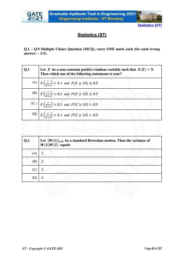
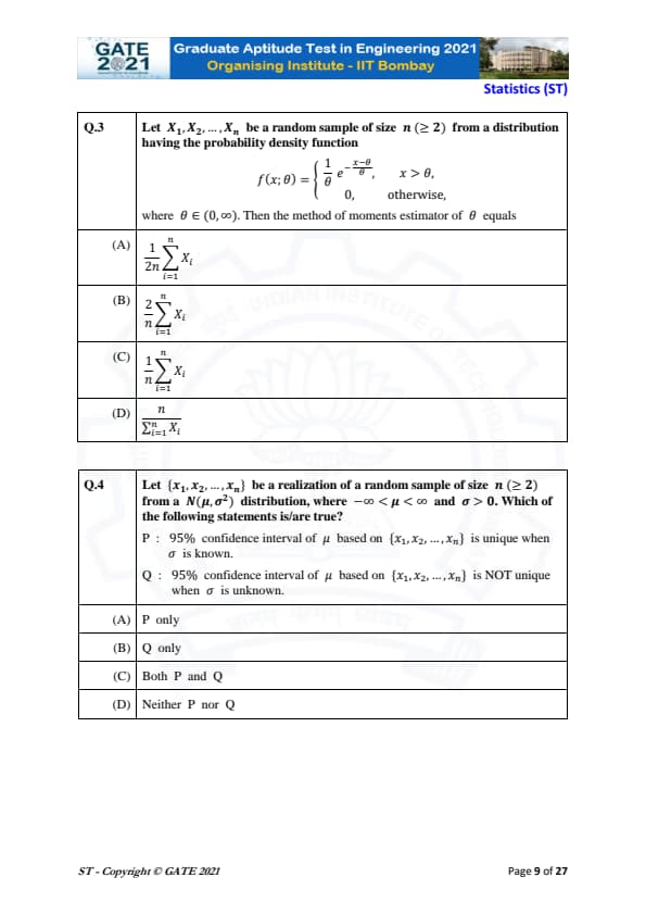
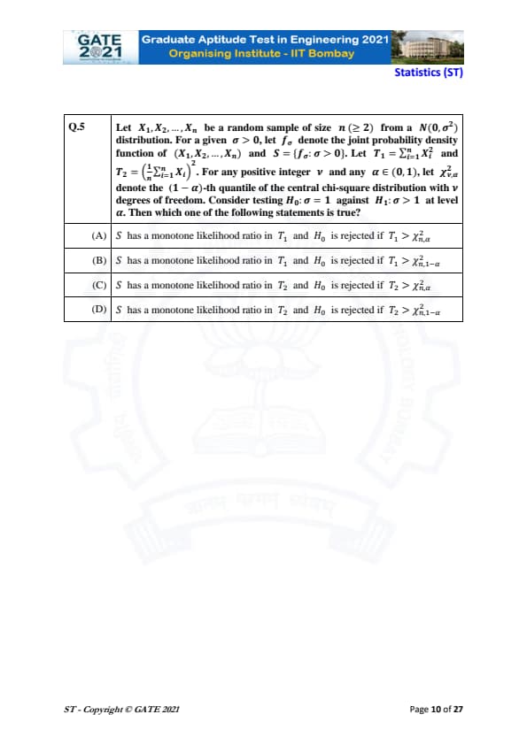
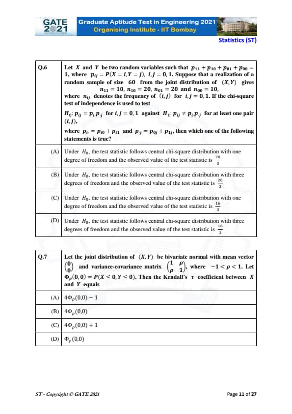
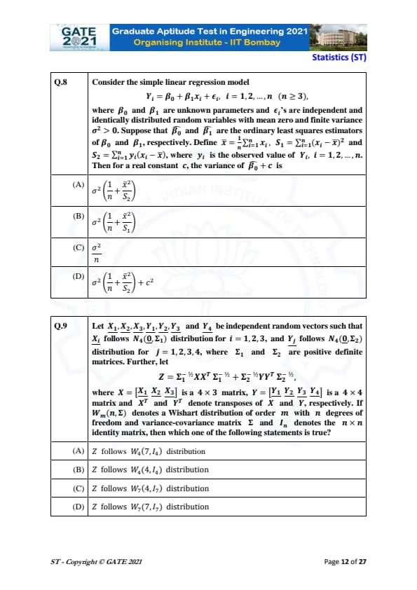
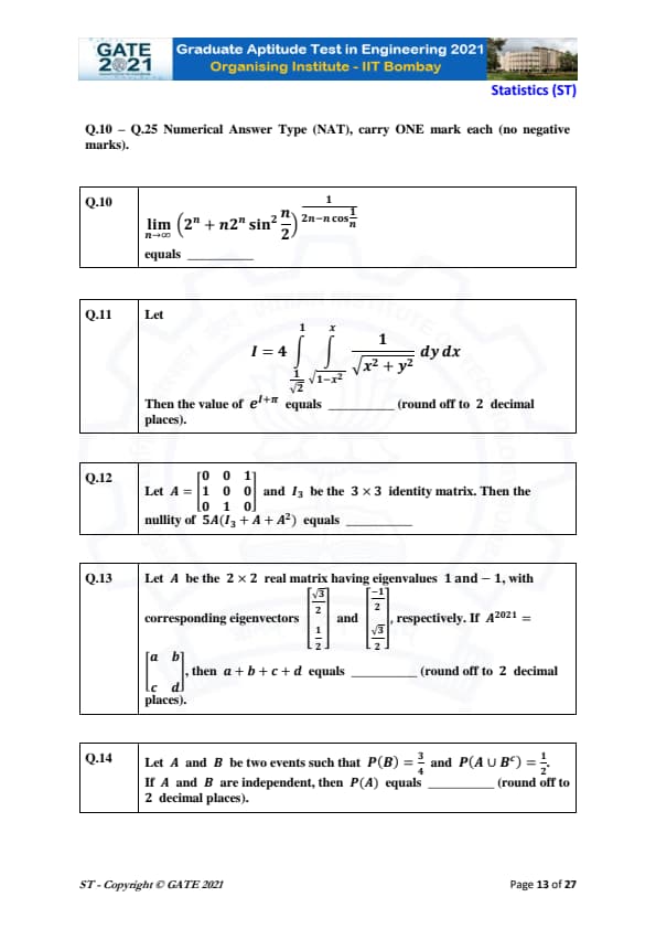
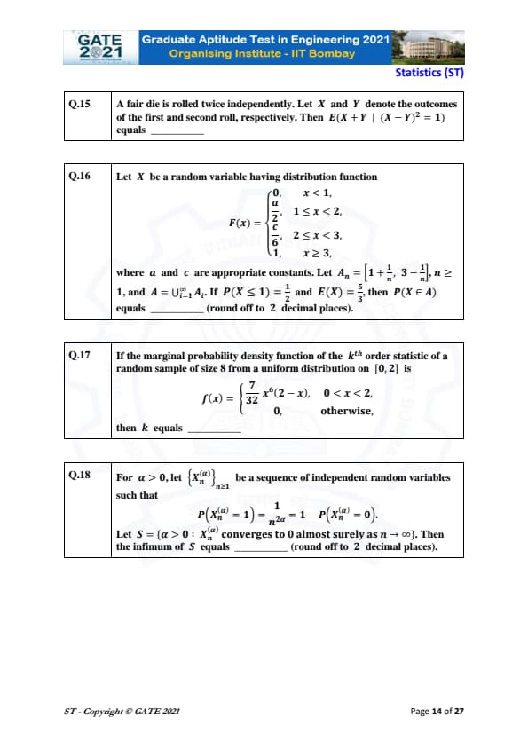
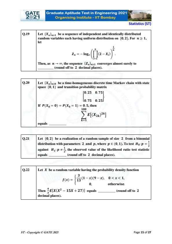
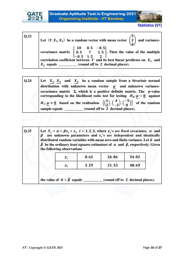
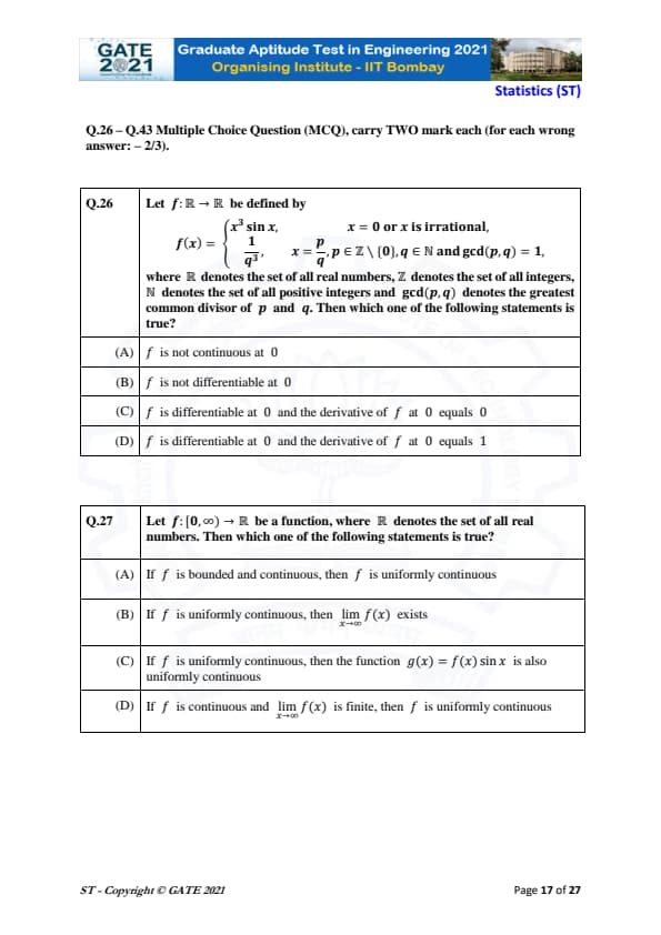
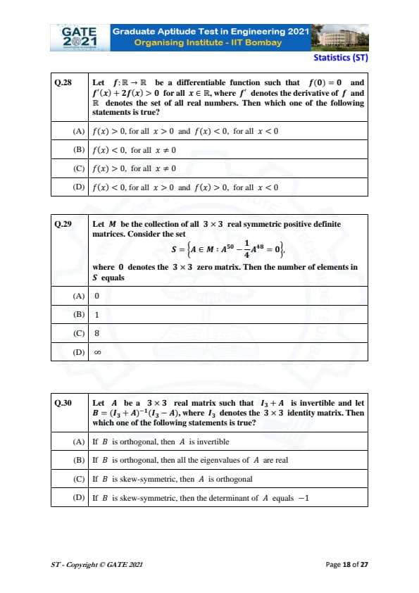
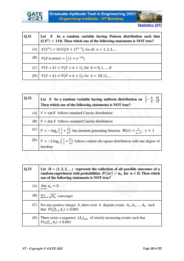
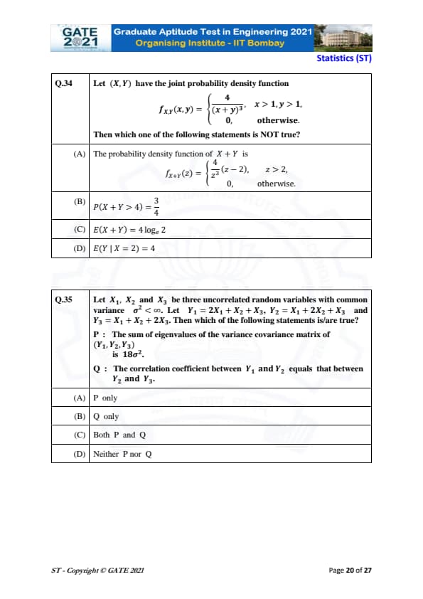
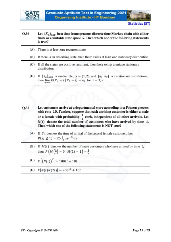
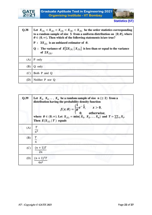
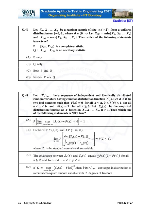
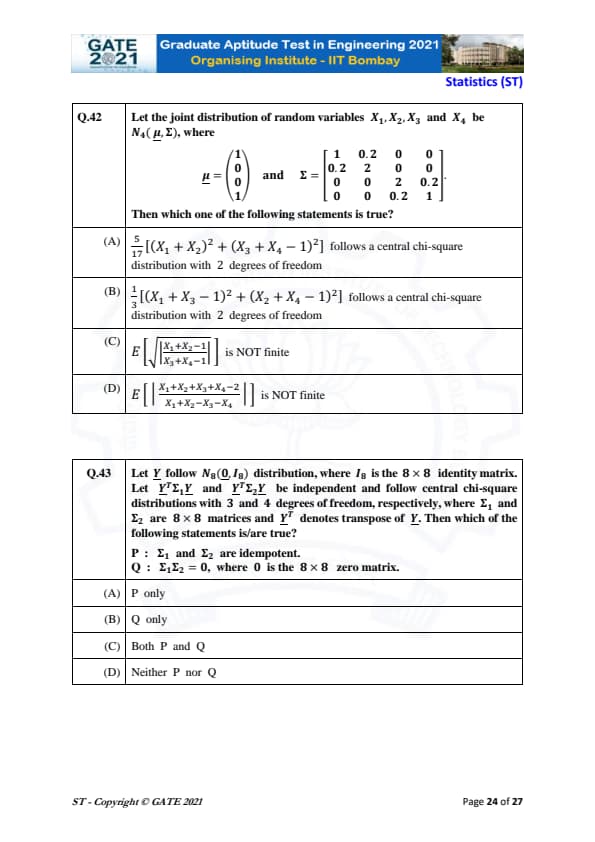
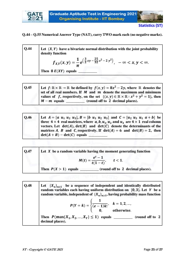
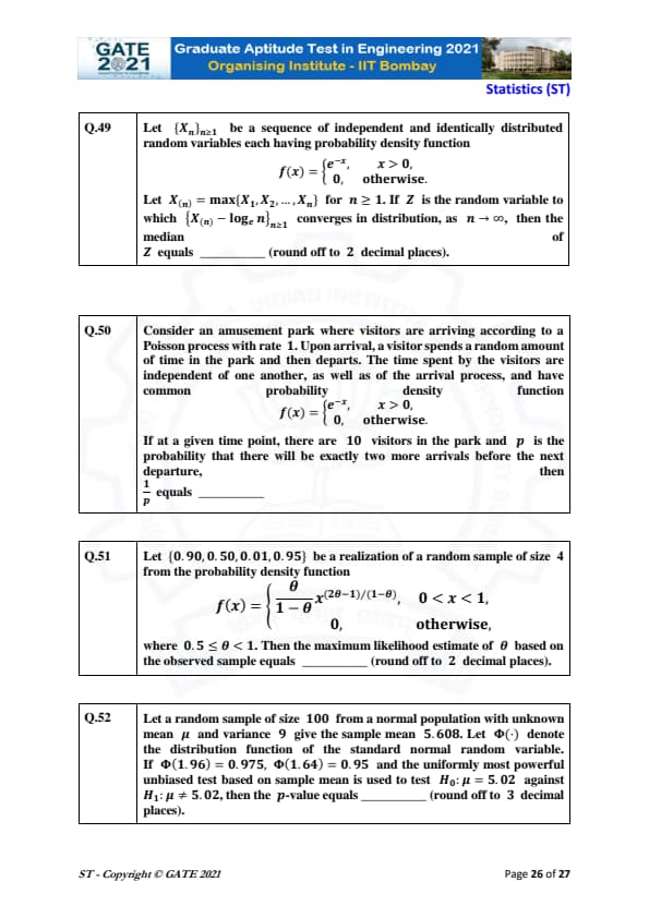
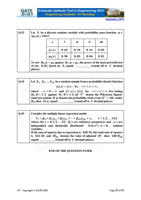
Quick Links:
GATE 2021 ST Paper Analysis
From 2021, IIT Bombay introduced MSQs. In MSQs, one or more than one correct answers would be mentioned in the question. A candidate is required to choose all the correct answers in MSQs to get the marks.
GATE 2021 ST was a combination of MCQs (Multiple Choice Questions), NAT (Numerical Answer Type) and MSQ (Multiple Select Questions). The full marks of the GATE 2021 ST stands at 100. All the questions carried either 1 or 2 marks. 180 minutes were allotted to solve 65 questions.
The table below shows the frequency of NATs, MSQs and MCQs carrying 1 and 2 marks, asked in GATE 2021 ST paper-
| Question Type | Question Frequency | Carried Marks |
|---|---|---|
| No of 1 mark MCQs/MSQs | 14 | 14 |
| No of 2 marks MCQs/MSQs | 23 | 46 |
| No of 1 mark NATs | 16 | 16 |
| No of 2 marks NATs | 12 | 24 |
Also Check:
GATE 2021 ST: Exam Pattern and Marking Scheme
- IIT Bombay concluded the exam in CBT mode
- Marks would be deducted only if MCQs were wrong. No marks would be deducted if any NATs and MSQs were proven to be wrong
- For every wrong MCQ carried 1 and 2 marks, ⅓ marks and ⅔ marks would be deducted respectively
- The qualifying cutoff goes up to 25 for Unreserved, 21.5 for OBCs, and 16.6 for SC/ST candidates
GATE Previous Year Question Papers
| GATE 2022 Question Papers | GATE 2021 Question Papers | GATE 2020 Question Papers |
| GATE 2019 Question Papers | GATE 2018 Question Papers | GATE 2017 Question Papers |
Comments